SVG SDFs
Little proof of concept to render SVGs with SDFs to get smooth and continuous distance fields for arbitrary shapes.
Signed distance fields keep popping up in my projects - lamps, vases, knitting patterns. The appeal is that a distance field turns a line into a landscape: every point in the plane suddenly knows how far away the drawing is and in which direction it lies. Here the drawing is an SVG - a logo, a sketch or the outline of a country - and that landscape is what gets colored. Everything on this page can be played with in the playground, load your own SVG and export the result as a PNG or as the raw buffer!

The Buffer
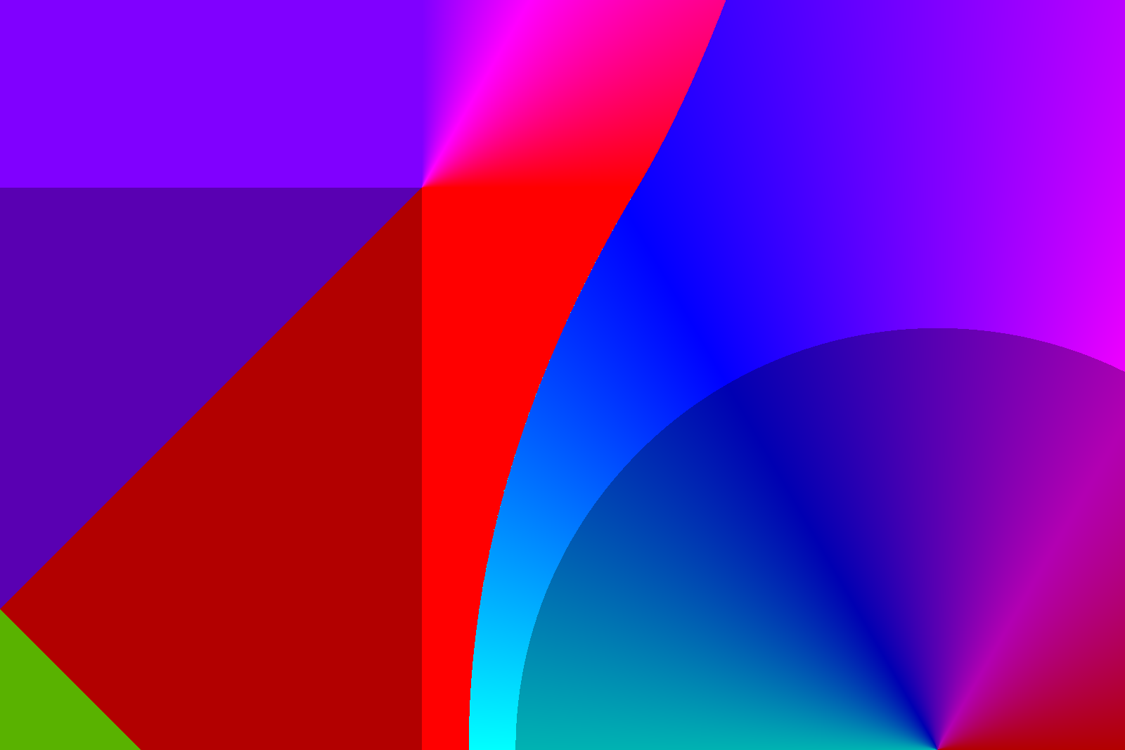
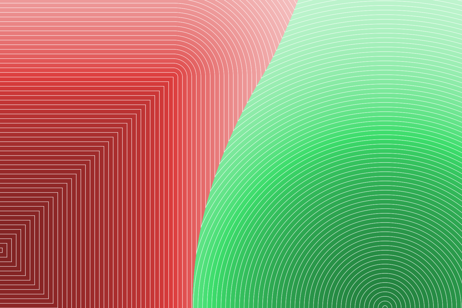
Every pixel of a fixed-resolution buffer stores four numbers: the signed distance to the nearest edge, the direction towards it and the shape it belongs to. That is the whole raw material, computed once.
Zoomed in on the gap between a square and a circle there is already quite a bit to see. The distance alone reads like a terrain, with a ridge running exactly halfway between the two. The direction cuts the plane into facets: flat bands along the straight sides, a fan around the corner and a sharp seam where the nearest edge jumps from one shape to the other. All coloring happens afterwards, so this is where the actual image making starts.

Distances
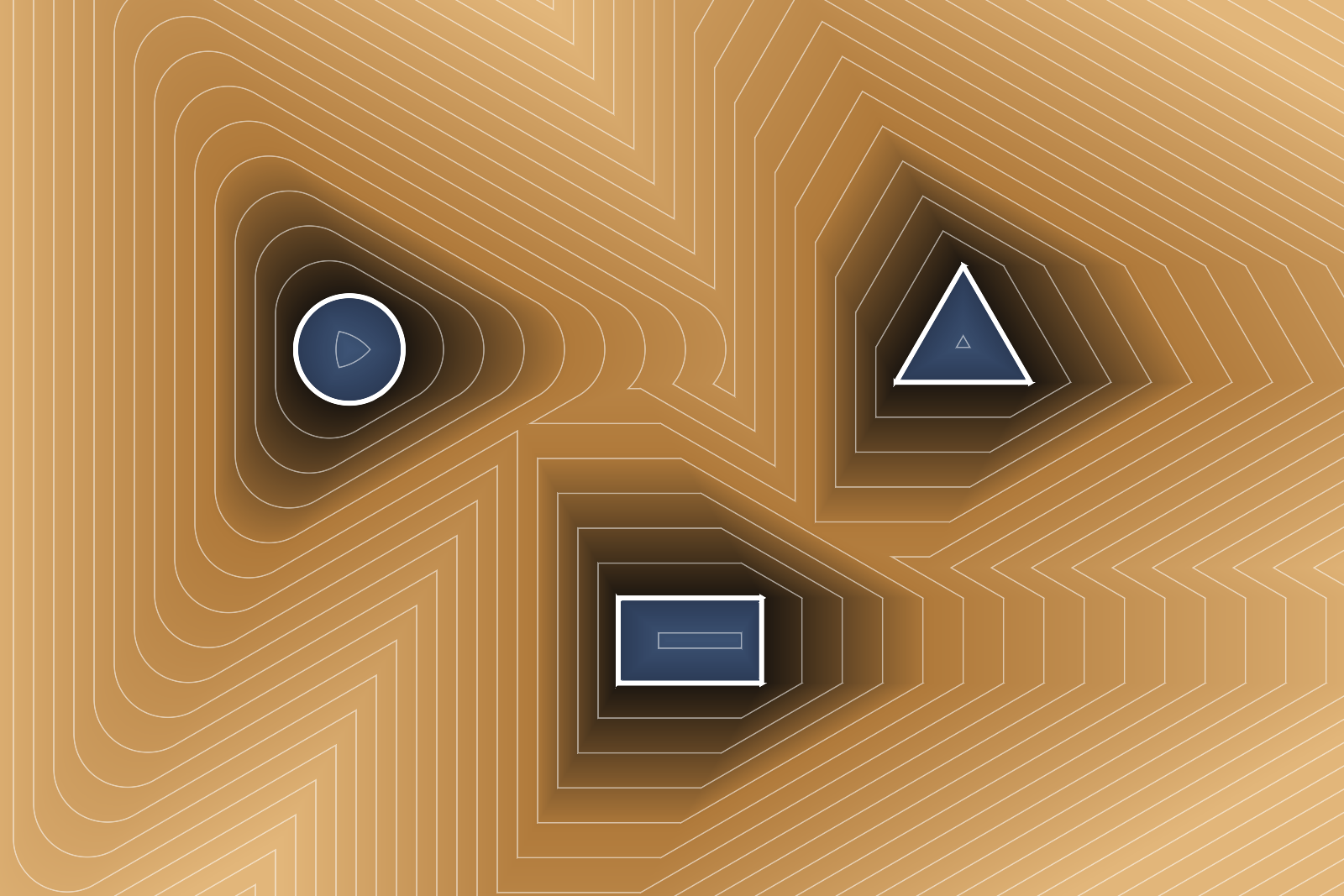
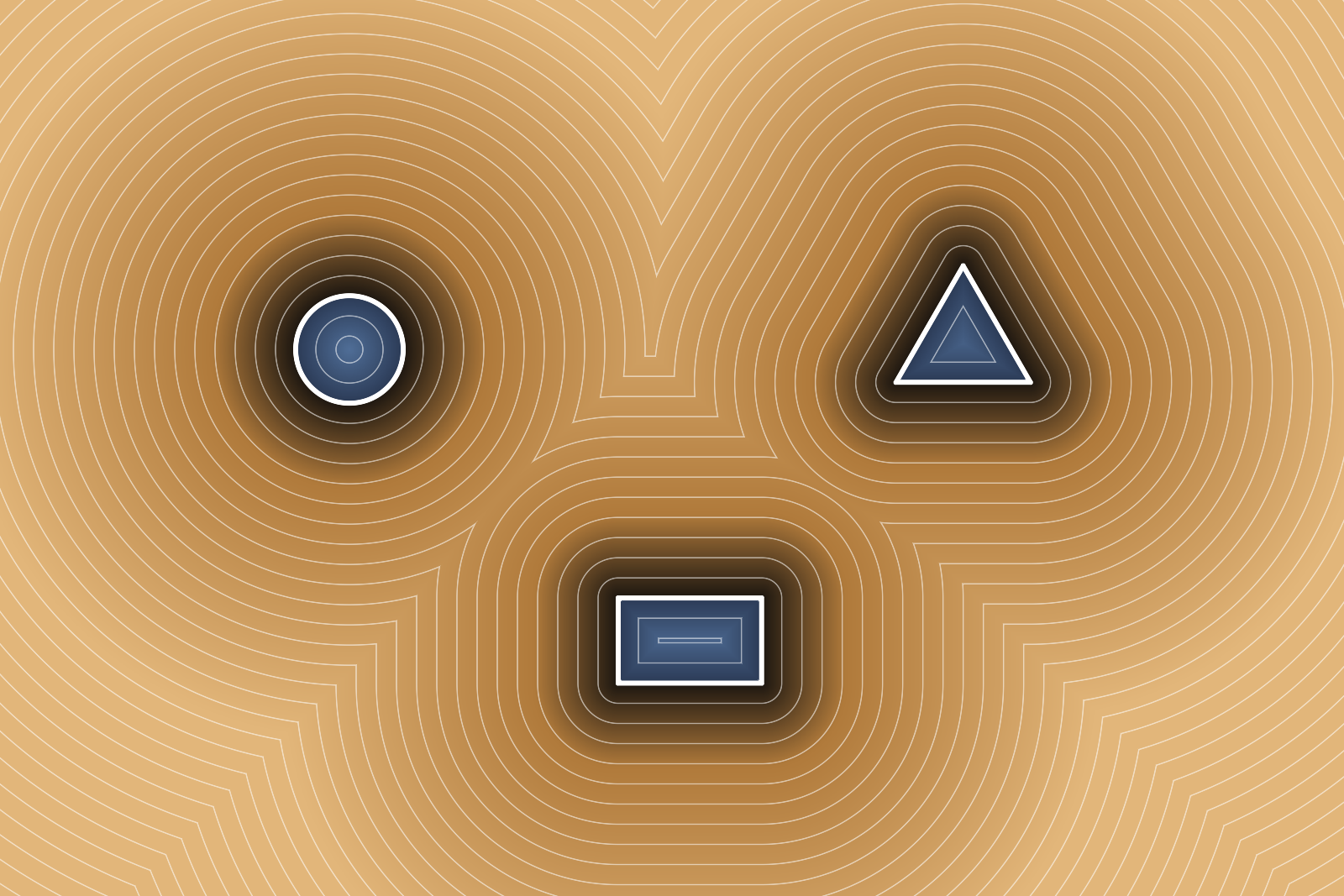
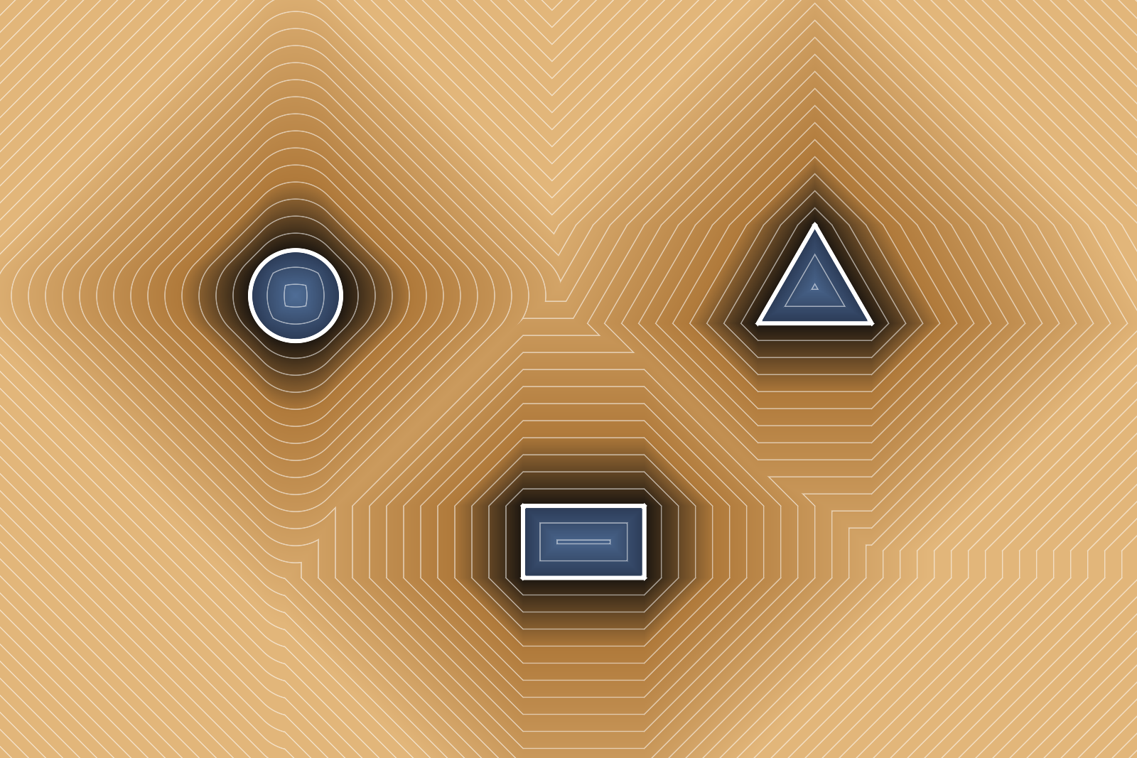
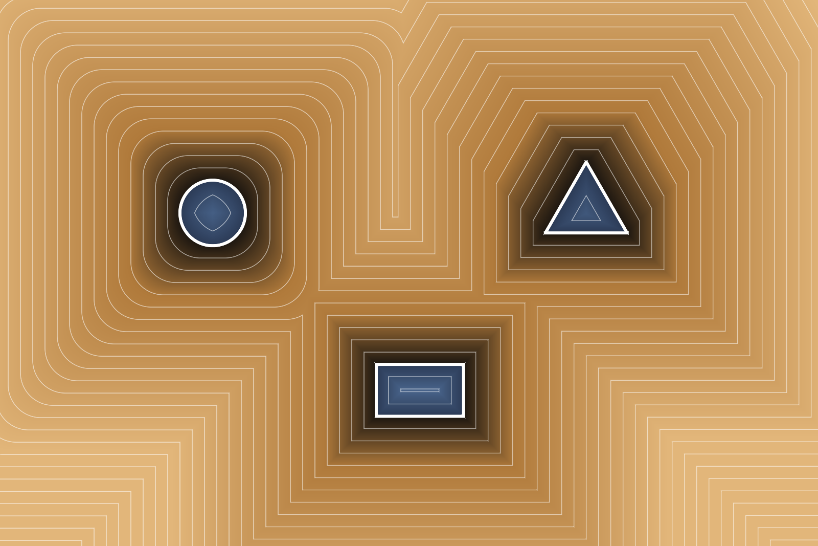
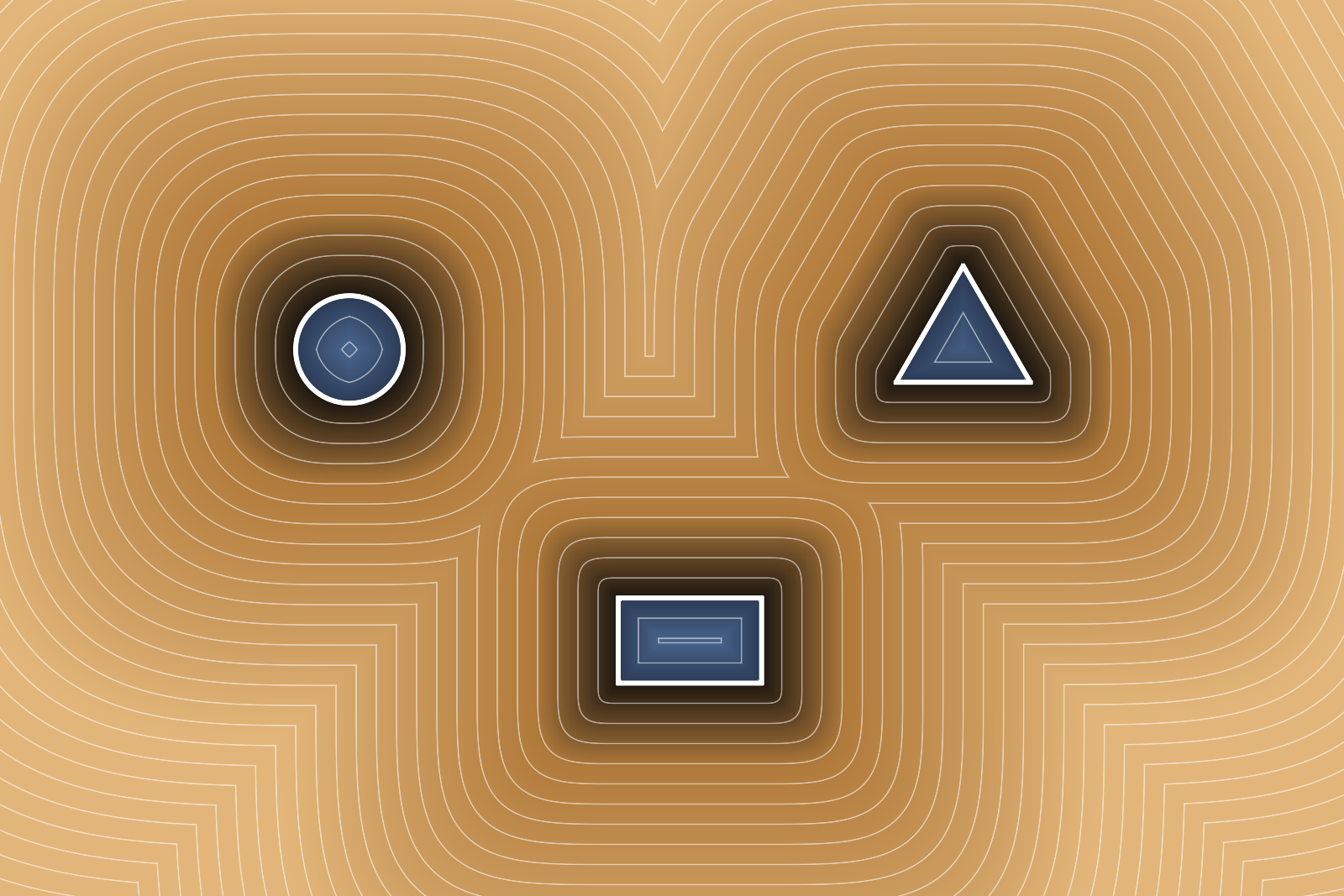
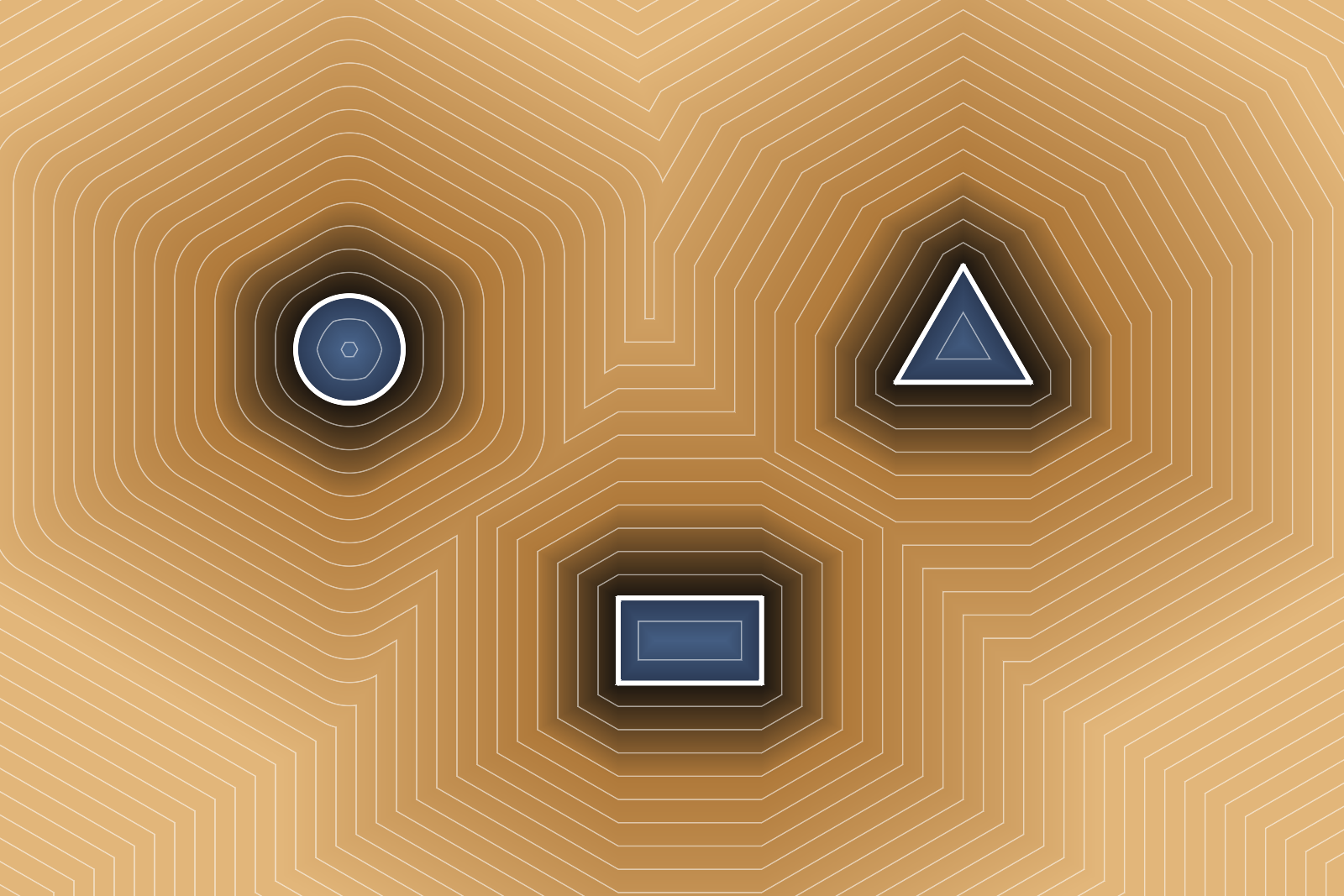
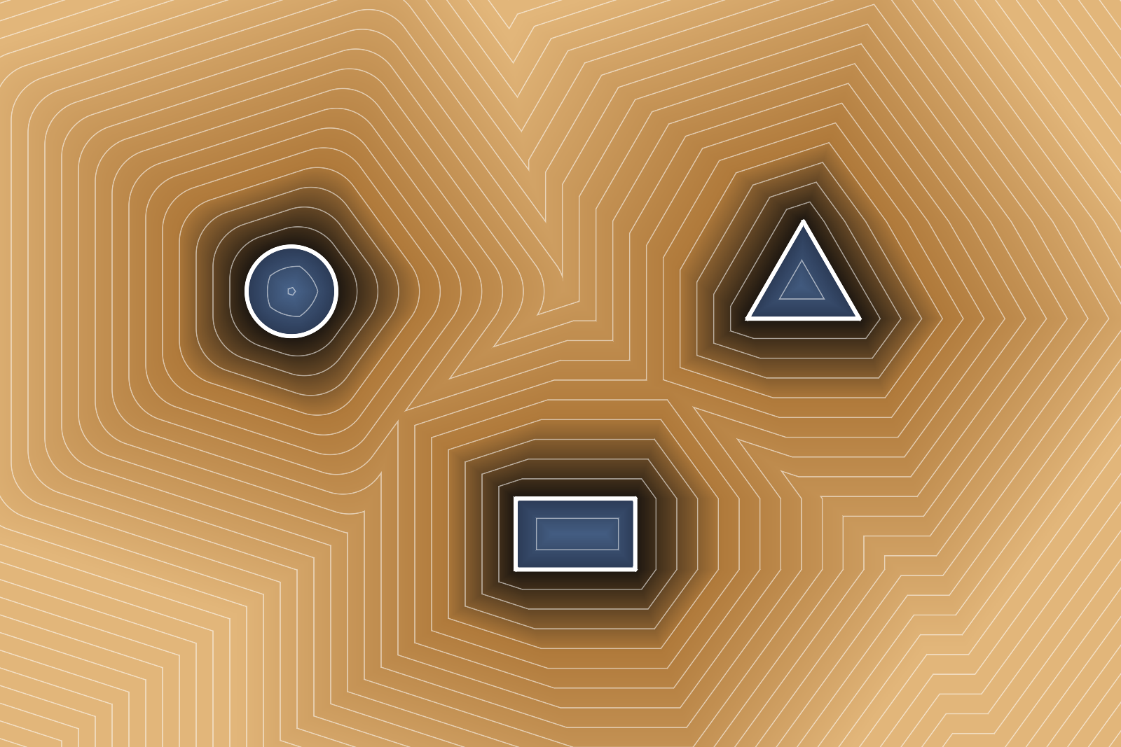
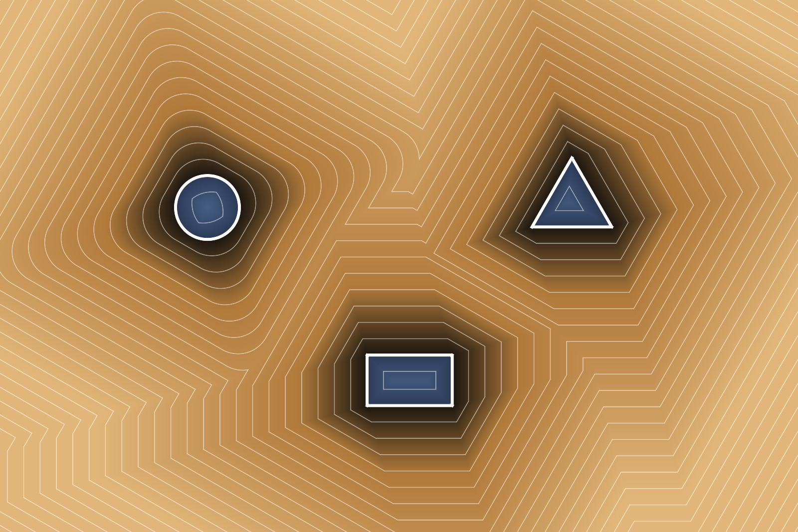
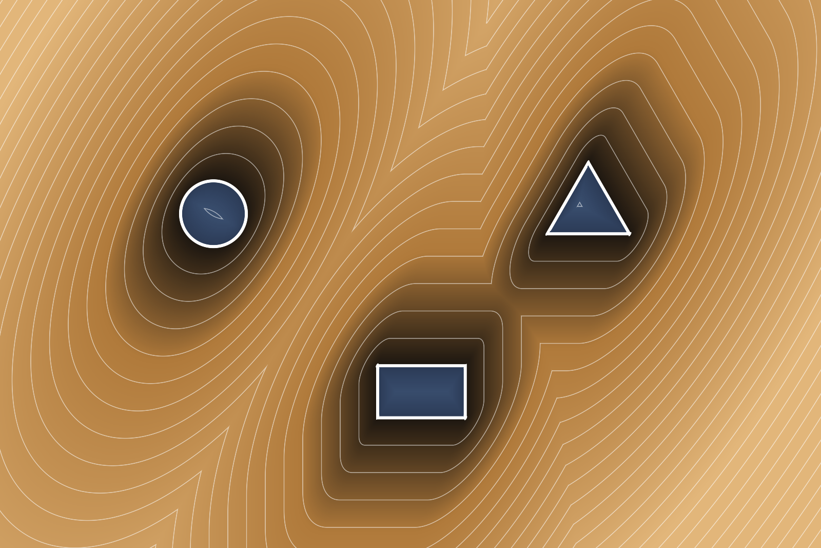
Euclidean distance is the obvious choice, but by no means the only one. Swapping the metric swaps the unit shape the distance is measured with: a diamond for Manhattan, a square for Chebyshev, anything in between the circle and the square for Lp and a regular polygon for the polygon metric.
Formally this changes quite a lot. Close to a shape the lines still follow its outline, further out they take over the formal language of the metric: soft and round for Euclidean, crystalline for Manhattan and Chebyshev, and rather wind-swept for the triangle and the pentagon, where the distance from A to B is not the same anymore as the one from B to A. Every metric can also be rotated and stretched, a stretched circle draws much like a slanted pen.
Curves
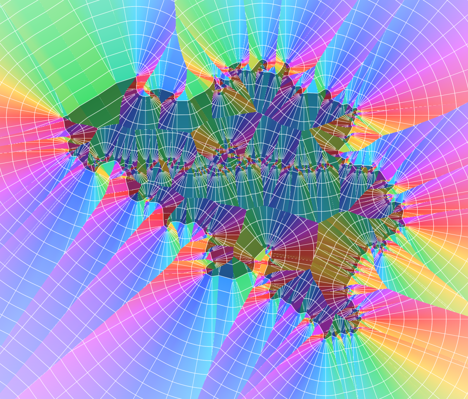
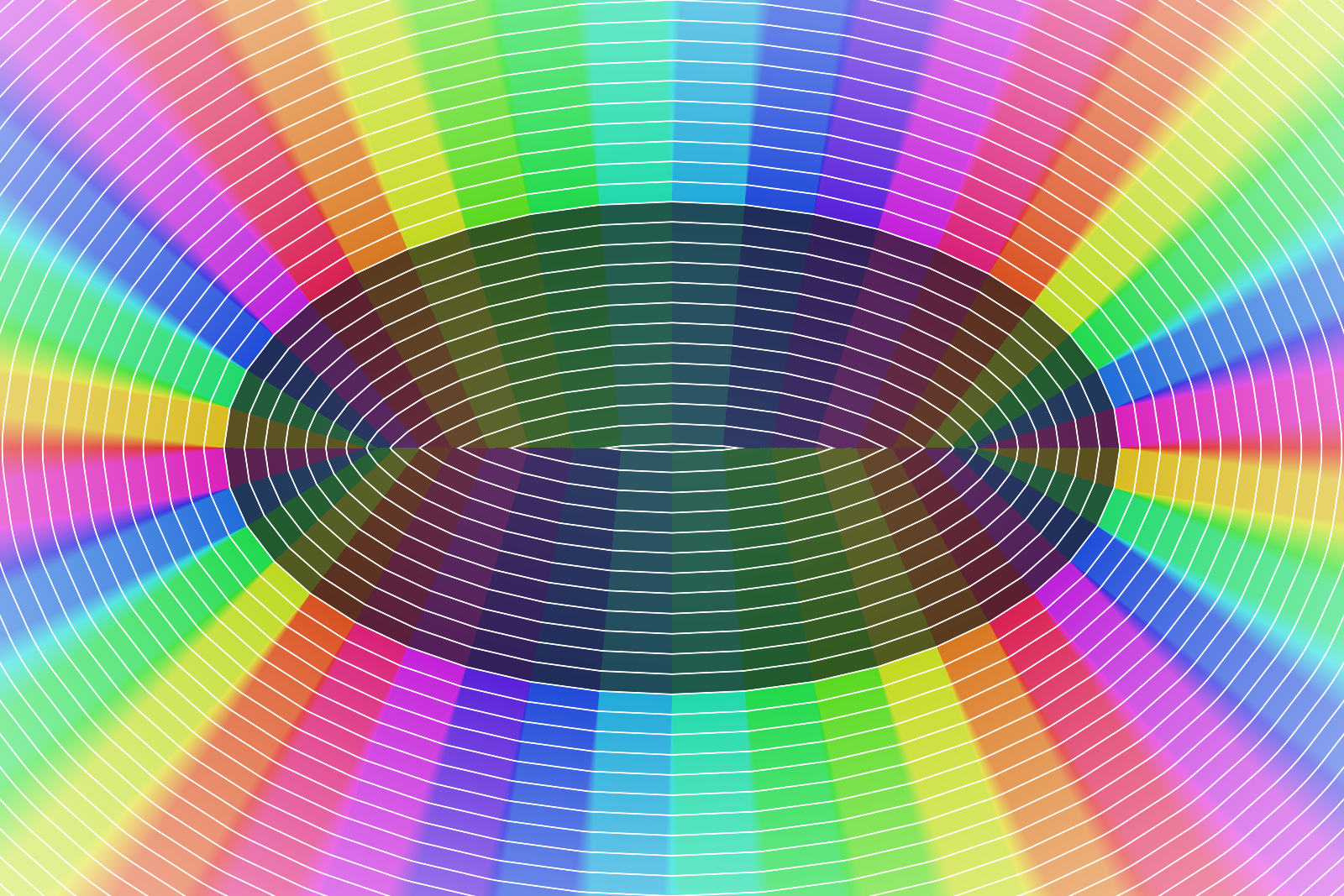
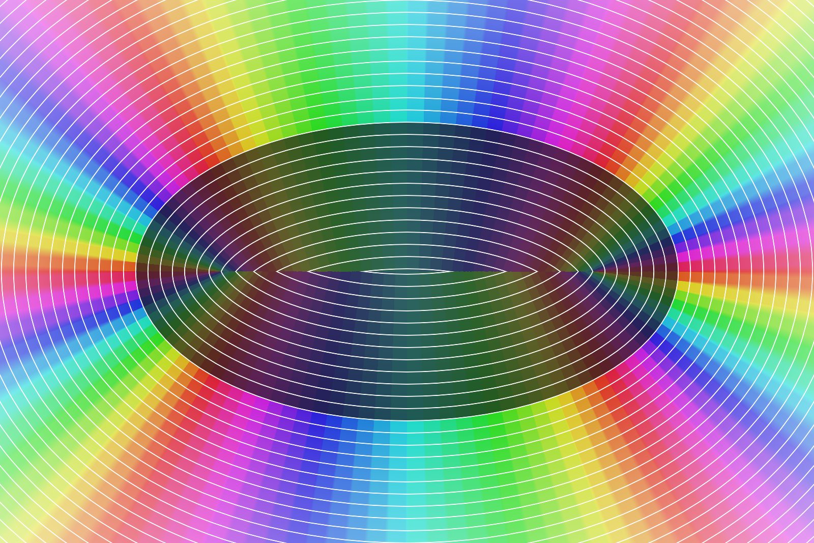
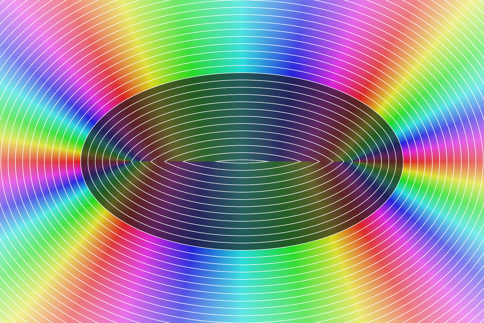
Curves can be flattened into polylines or kept as cubic Béziers, with the distance measured to the actual curve. Flattening is cheap, though the direction to the nearest edge is then constant along every straight piece, which shows up as hard bands as soon as you color by direction.
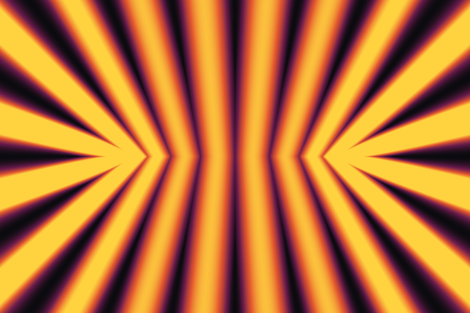
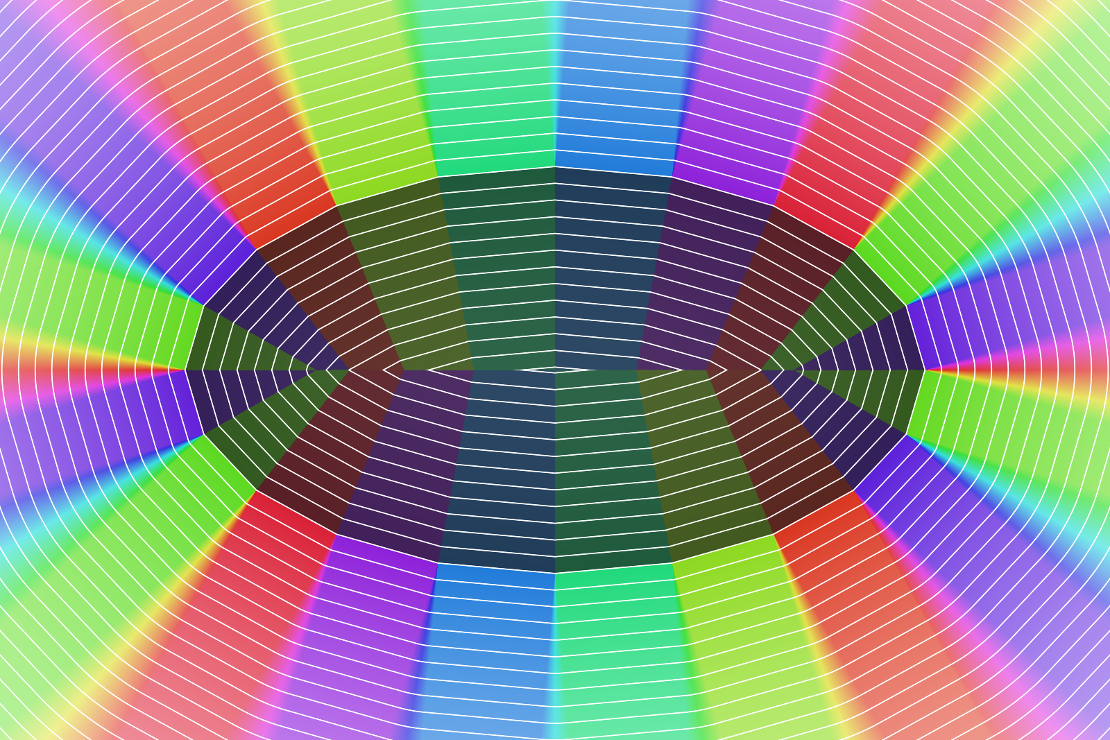
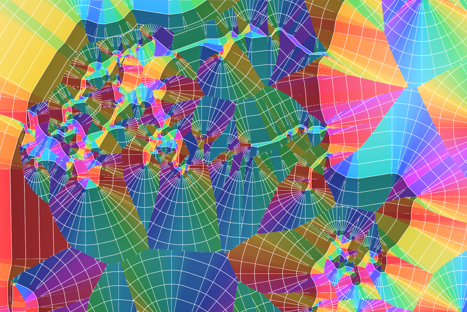
Though the bands are not only an error, they are a texture of their own. On the ellipse below the hue goes round six times per turn: a polyline that may be 8 pixels off gives faceted fans, 2 pixels gives finer ones, a quarter of a pixel is almost smooth and the exact curve completely so. The image next to this text only shows the difference in distance between the coarse polyline and the exact curve - an error map basically - and it turned out to be the prettiest image of the lot.
Post-Processing
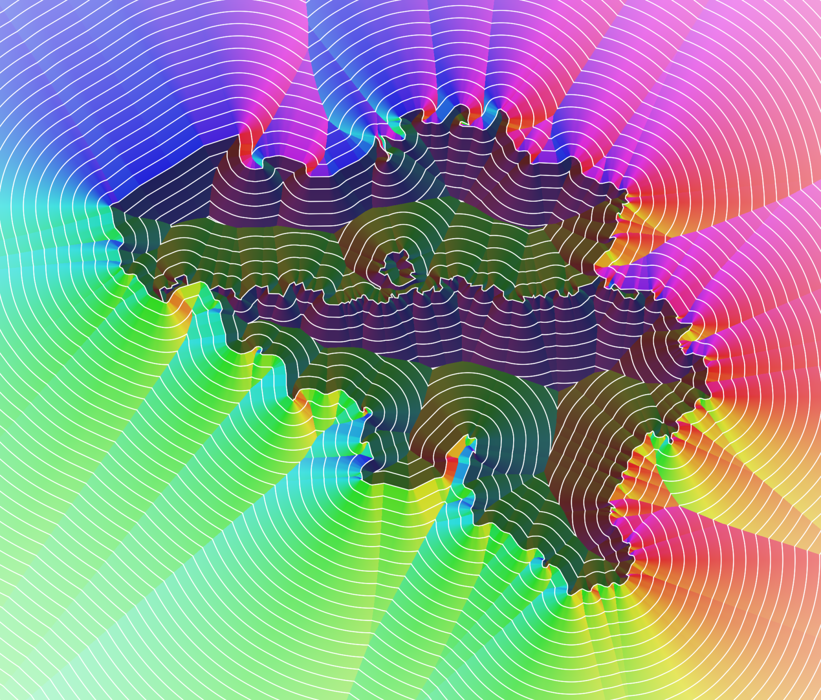
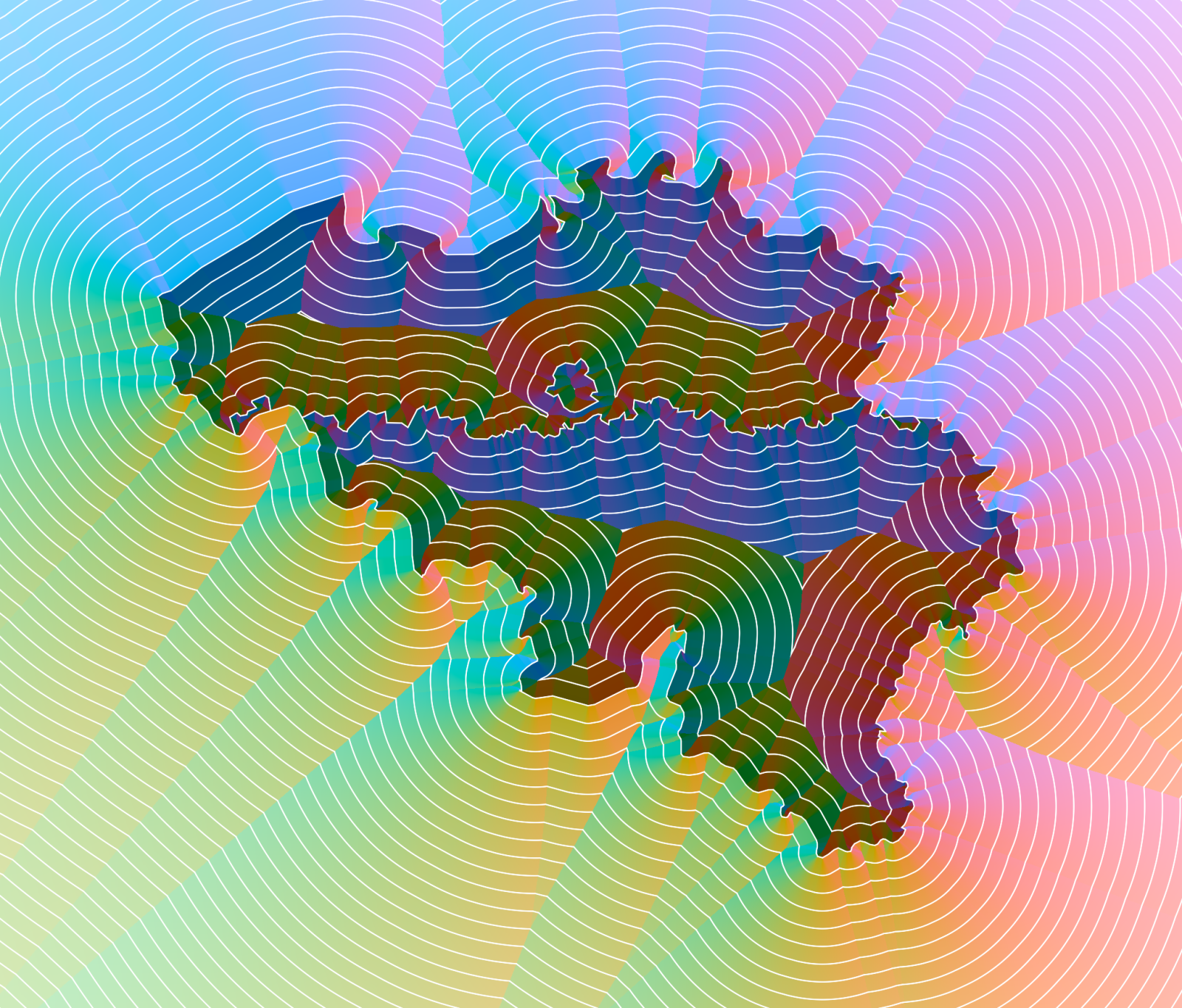
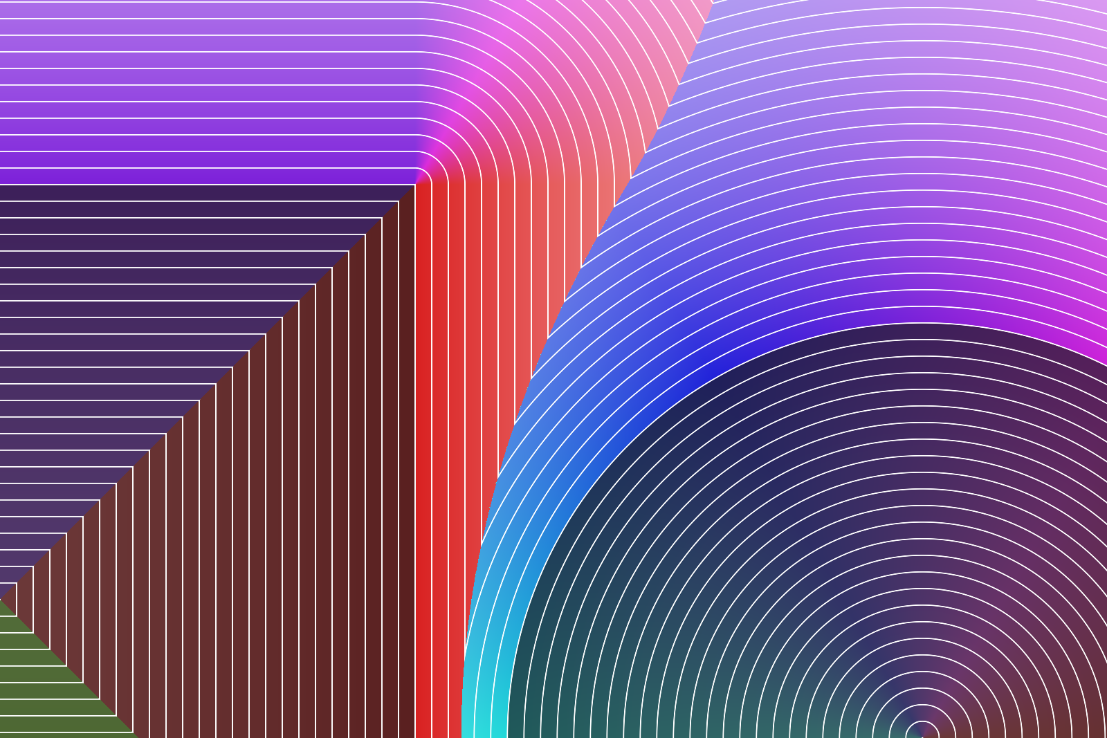
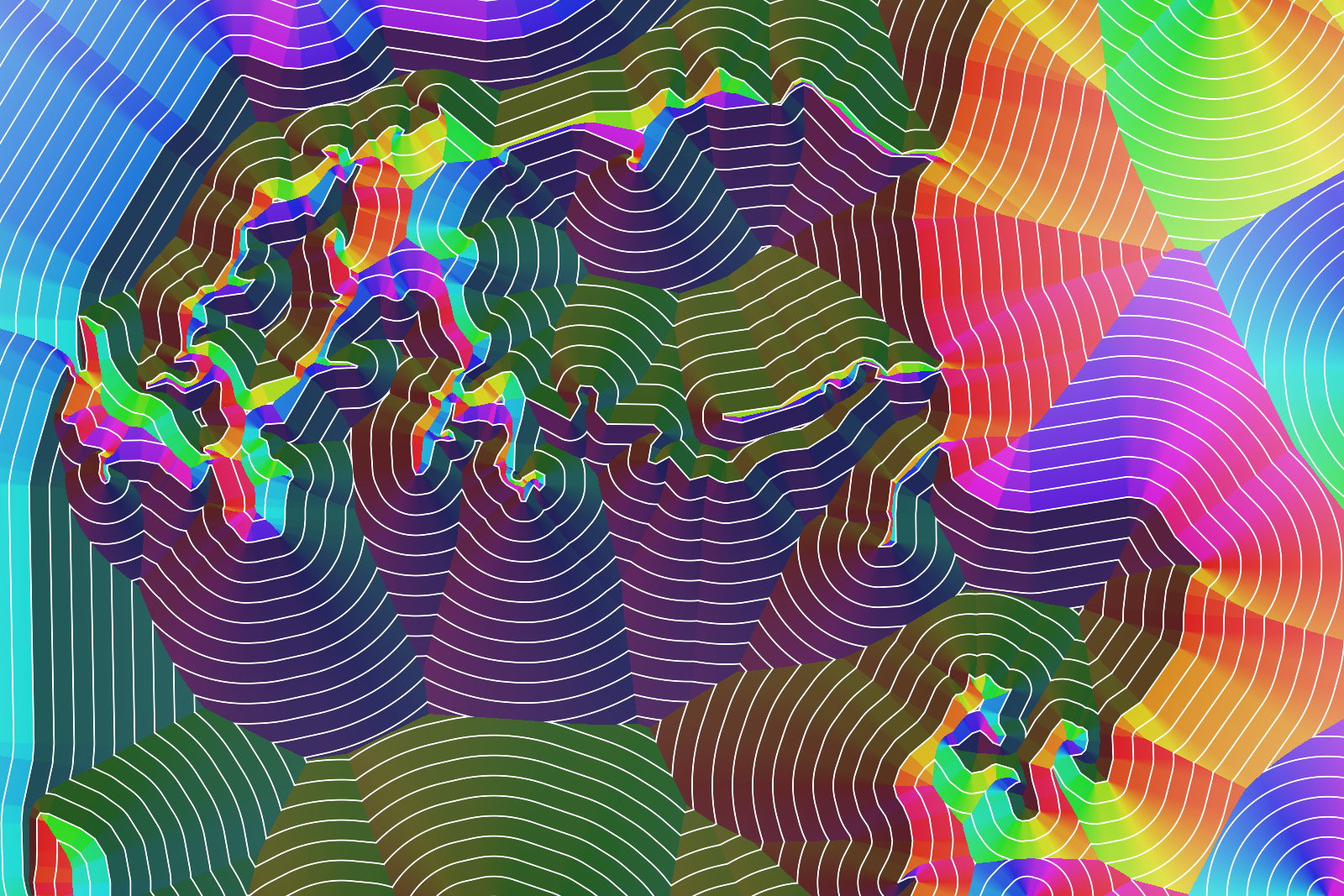
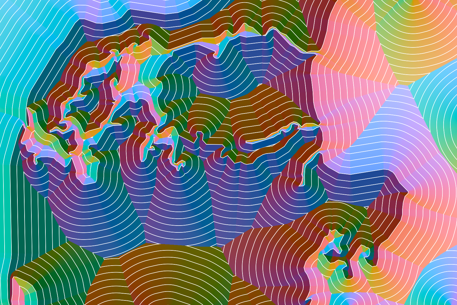
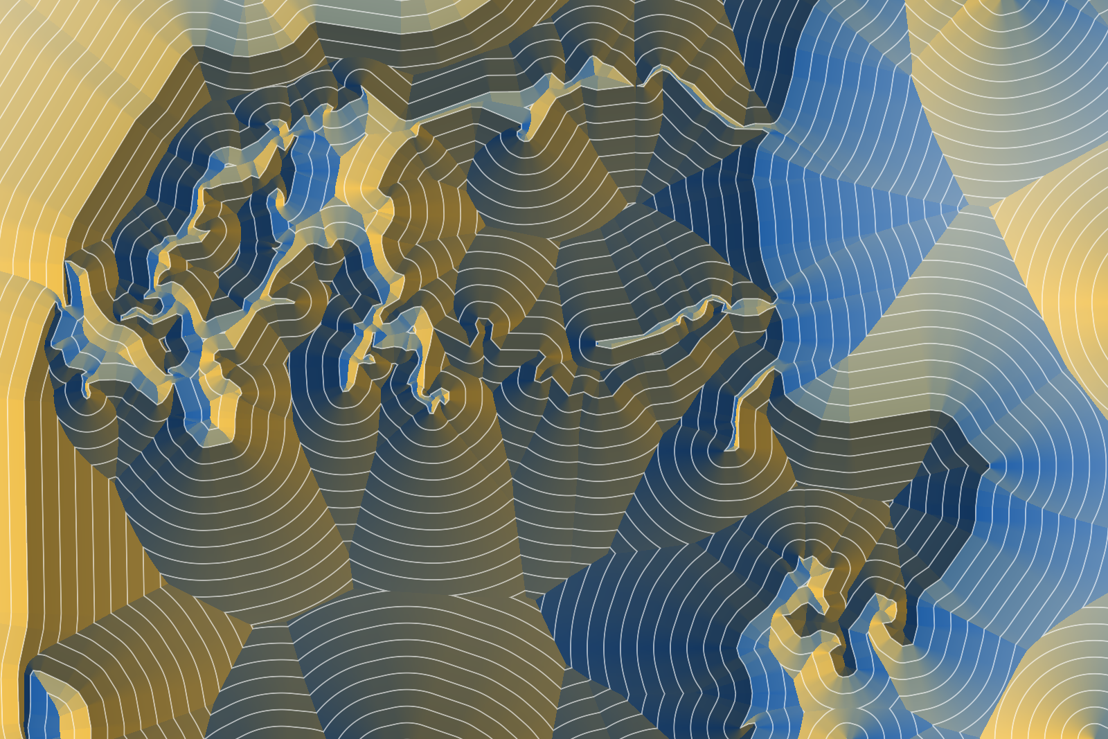
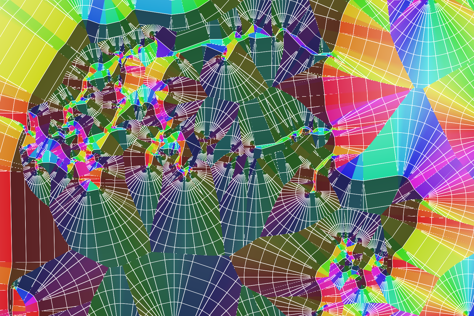
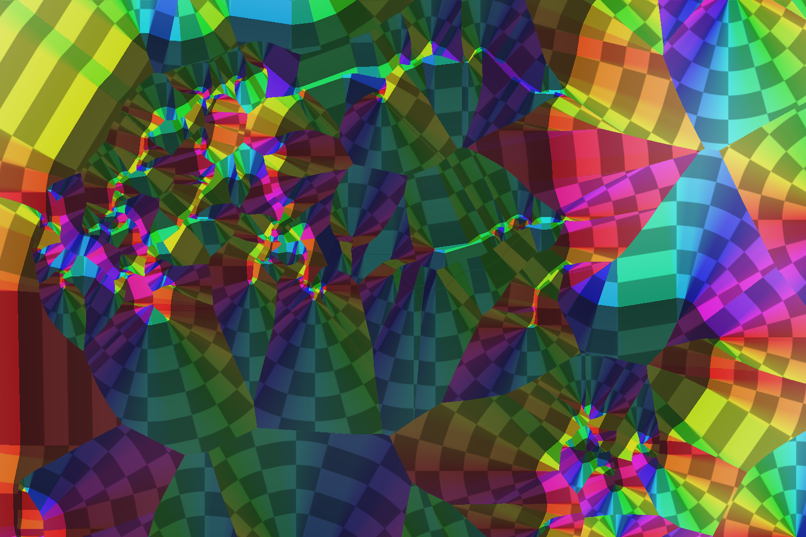
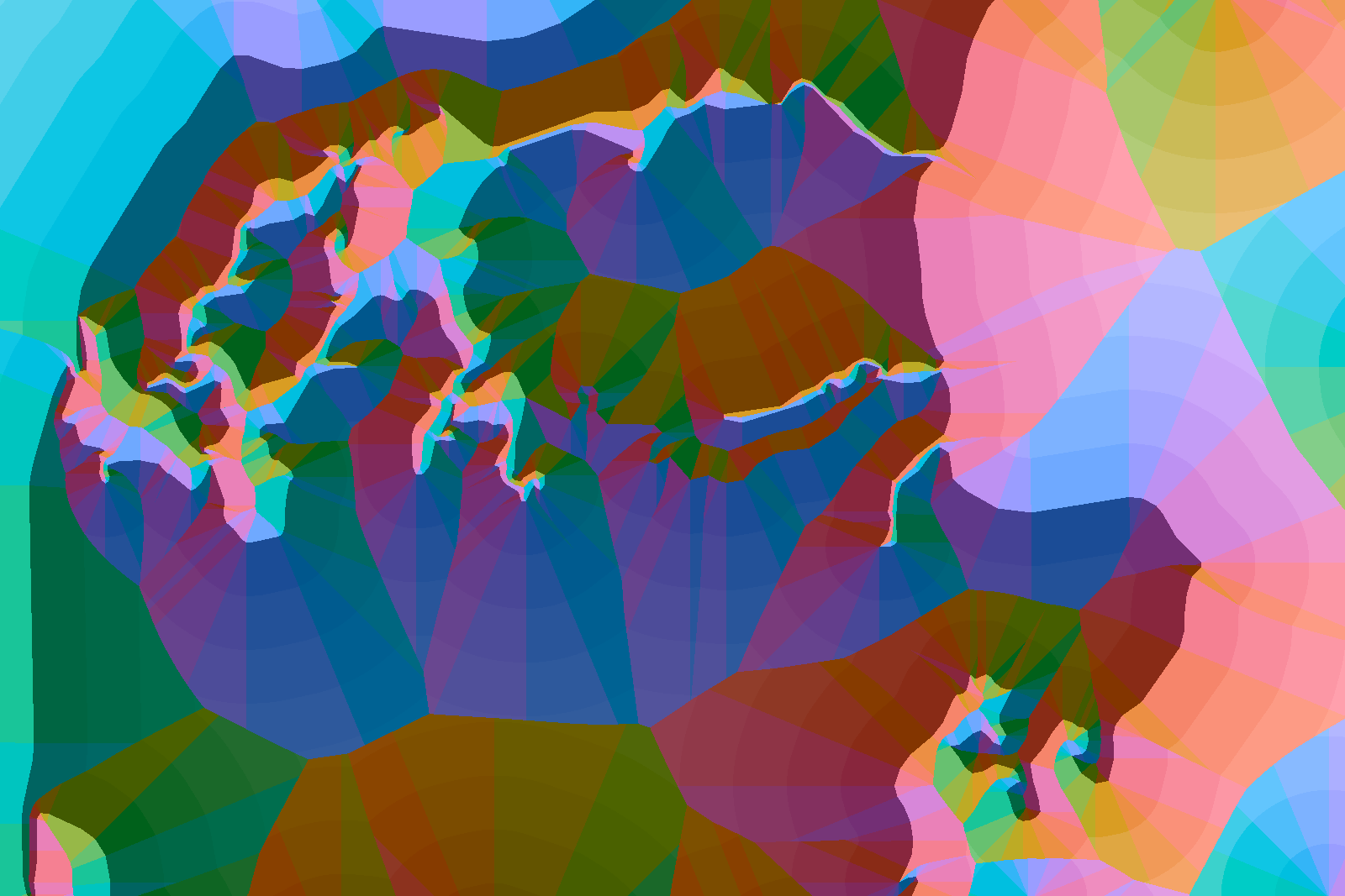
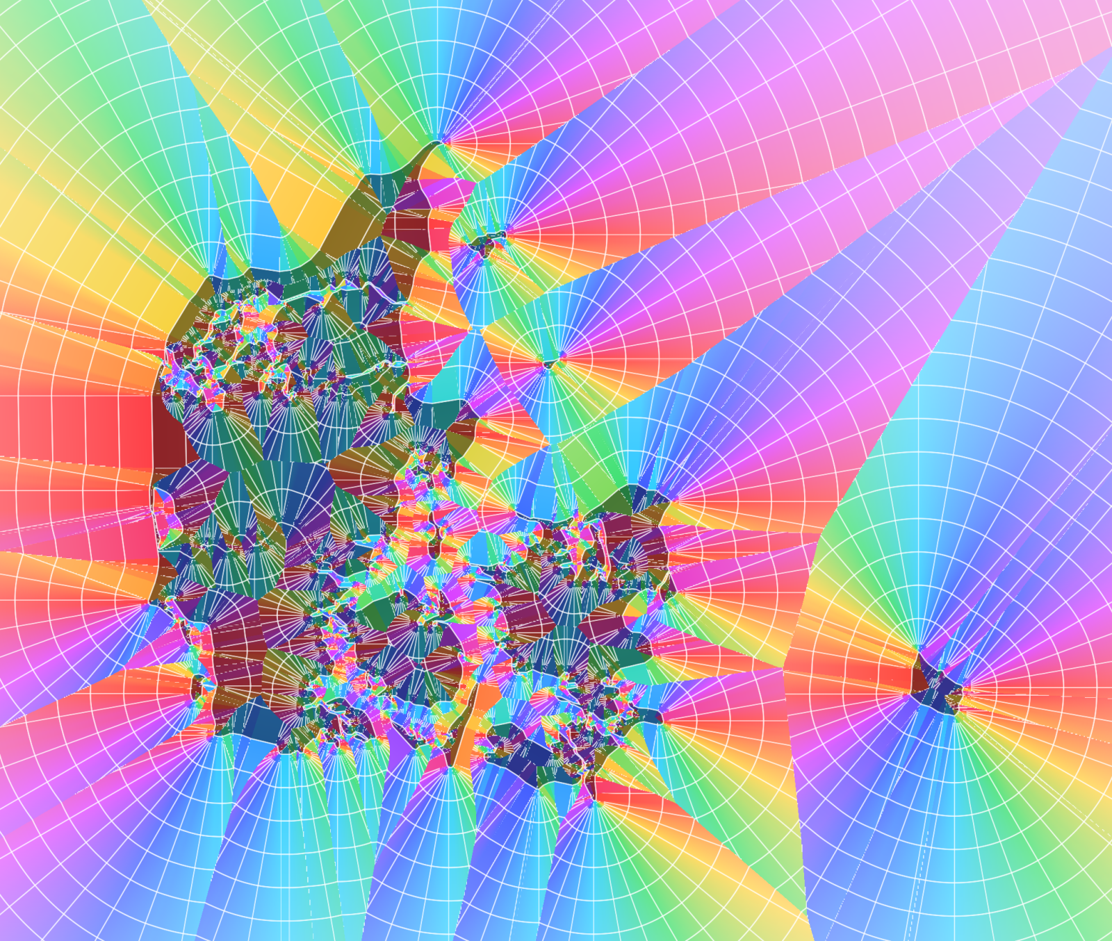
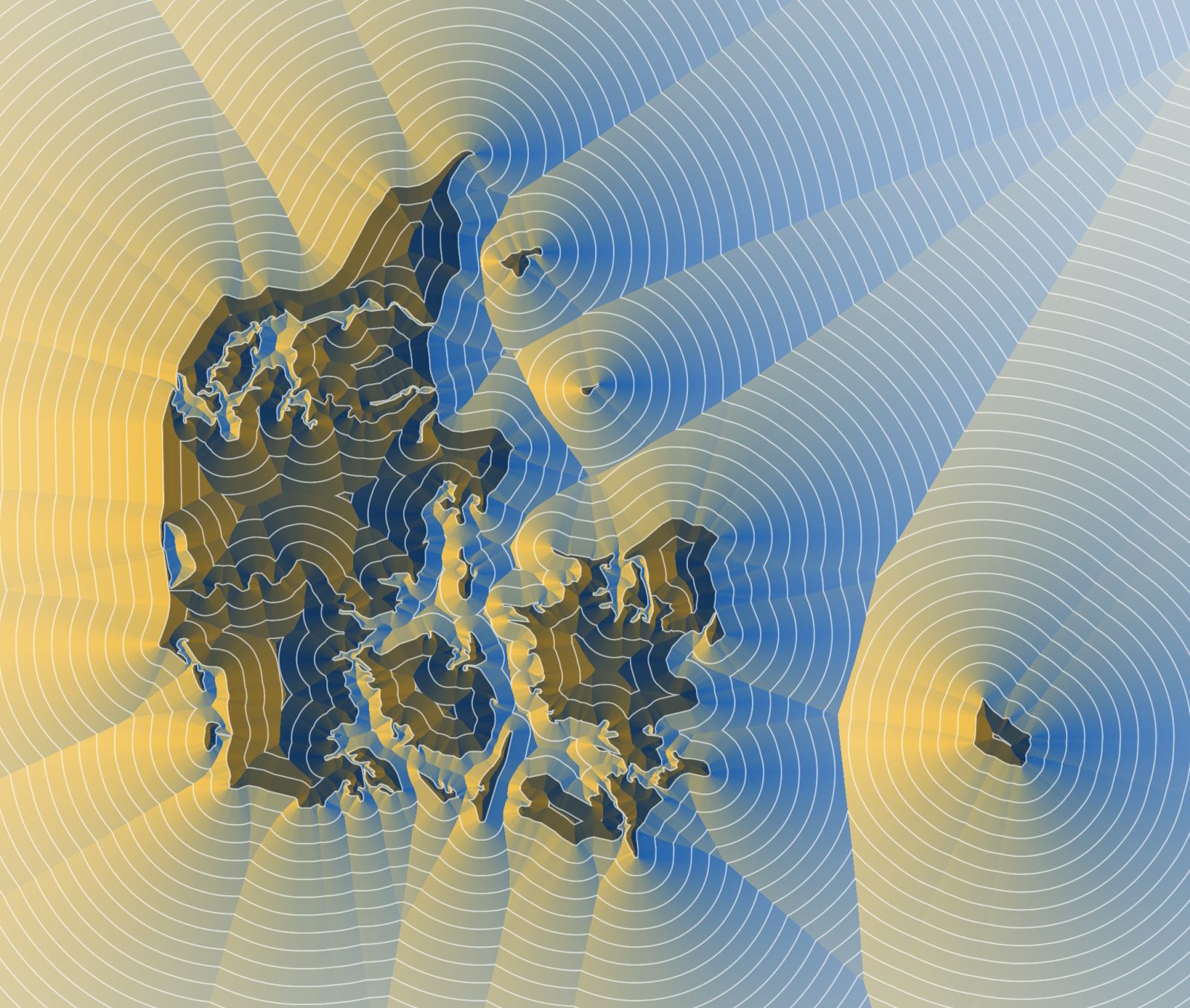
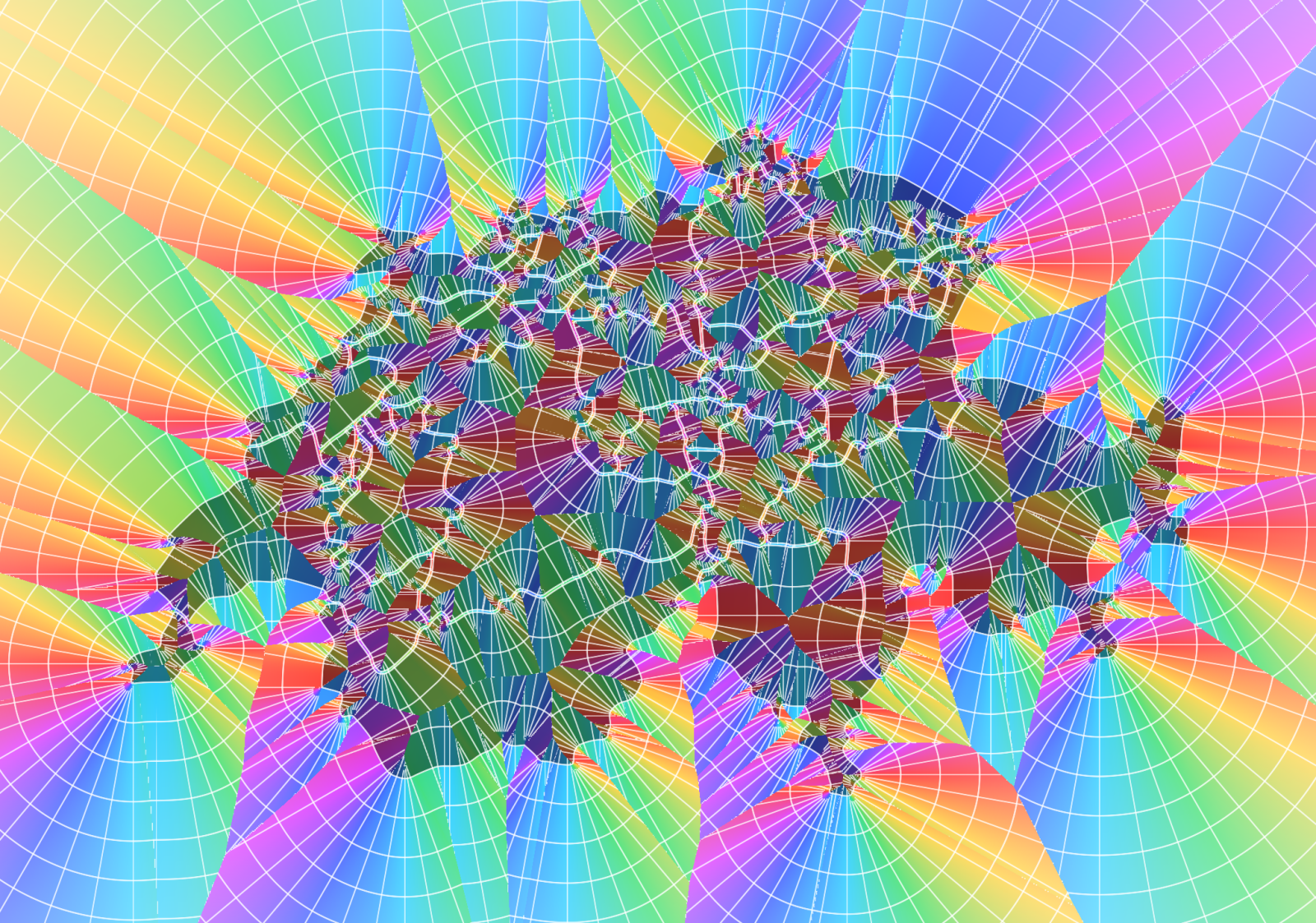
One buffer, a whole bunch of images. The polar mode reads the field like a compass: the hue comes from the direction to the nearest edge, its strength from the distance. The hues come from an HSV rainbow, a perceptually even OKLCH wheel or a cyclic gradient of your own, with radial lines, a checker or a mosaic of tiles on top.
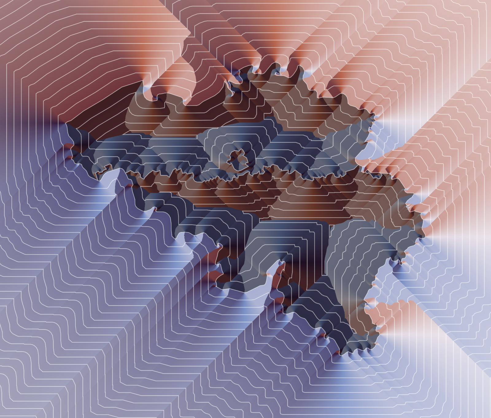
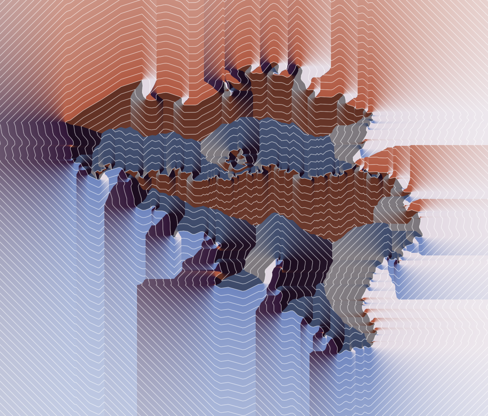
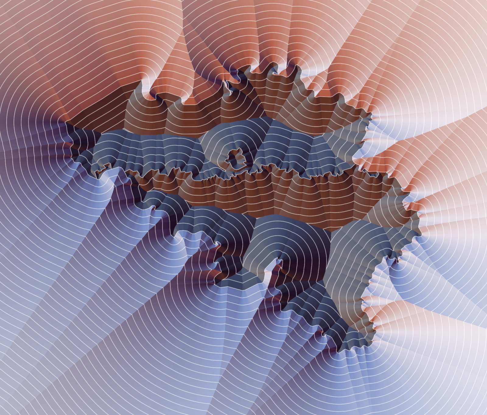
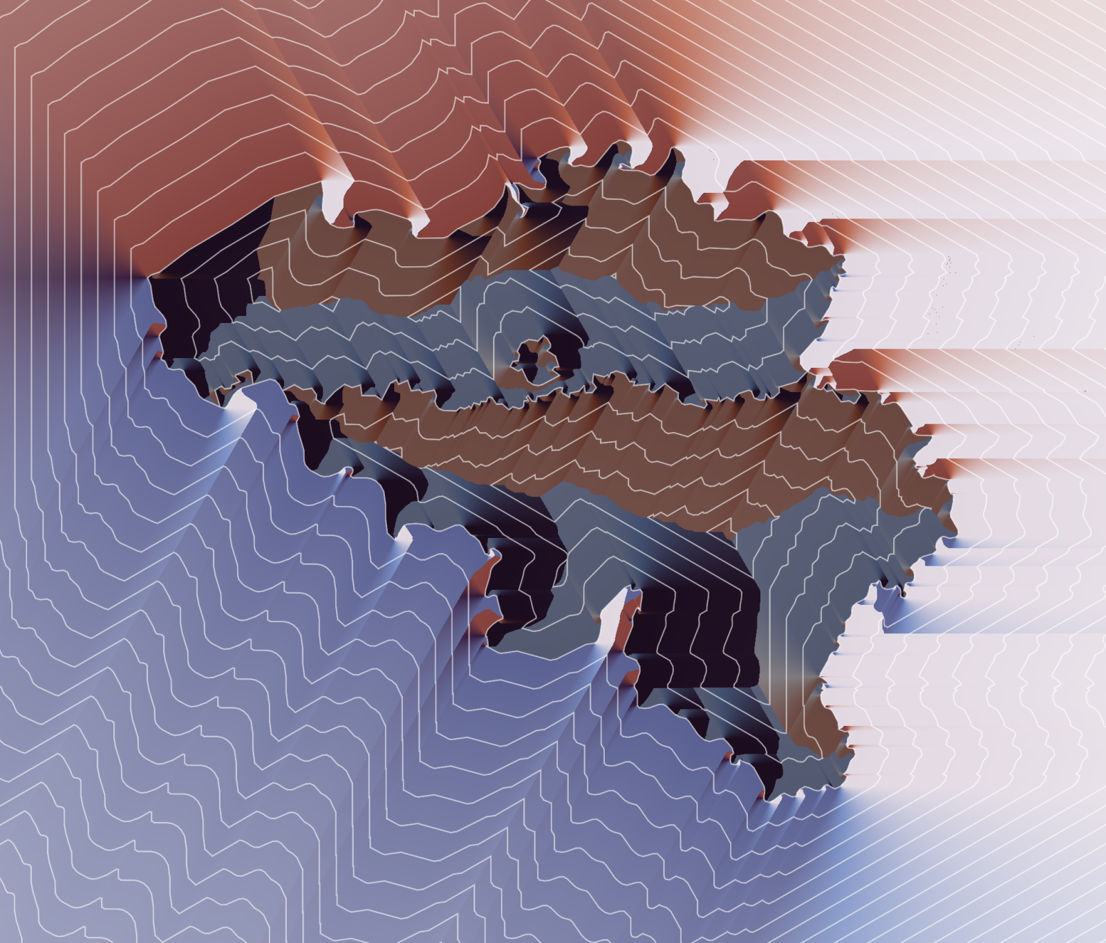
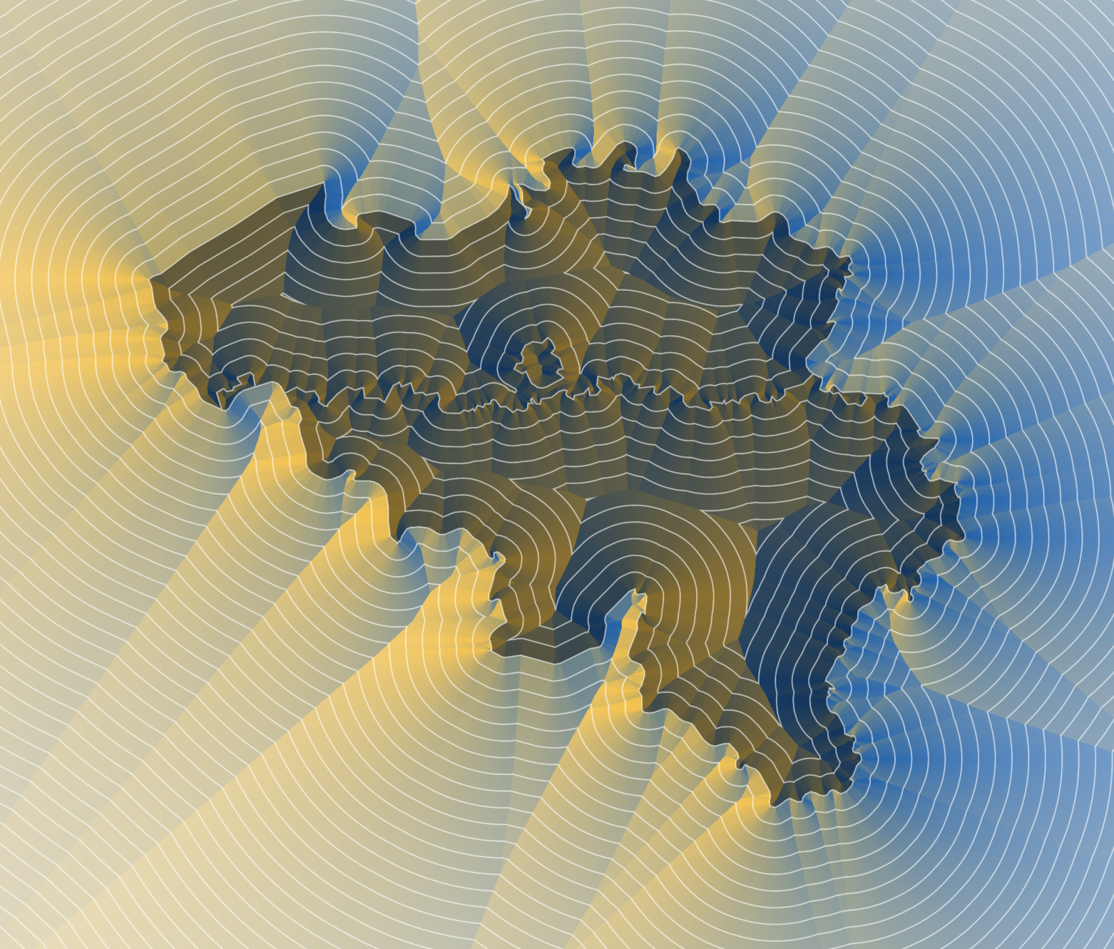
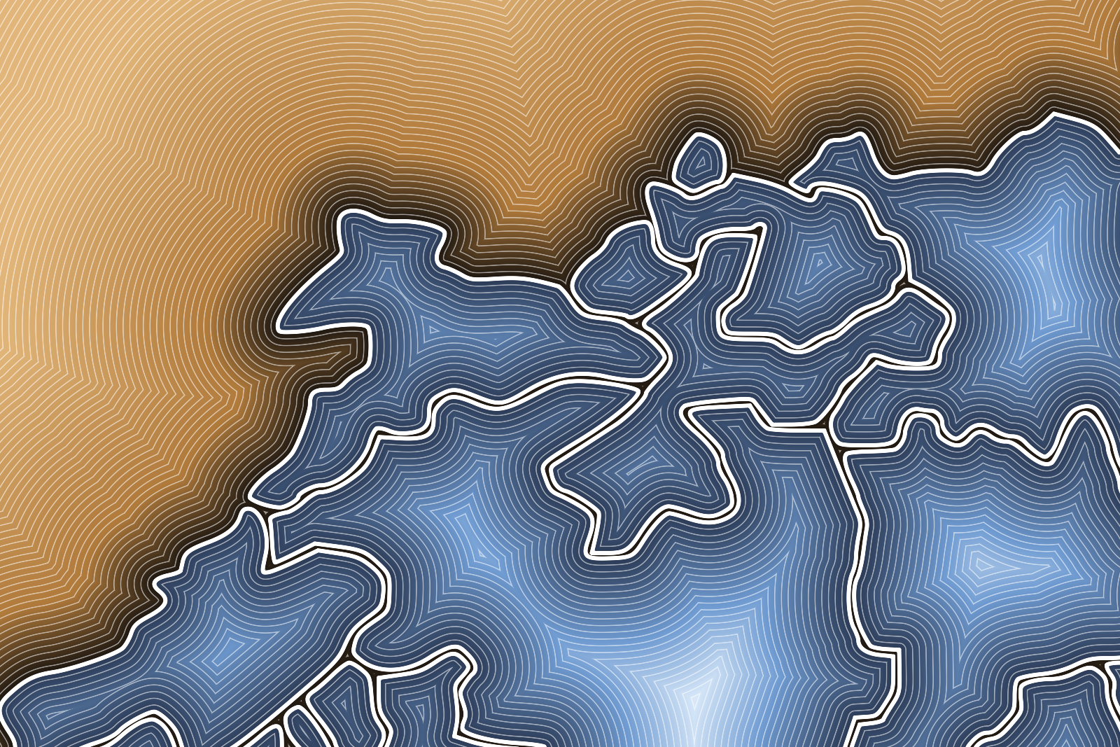
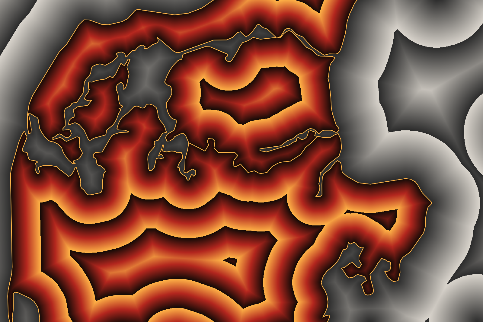
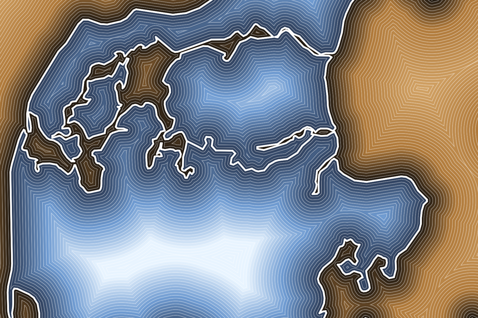
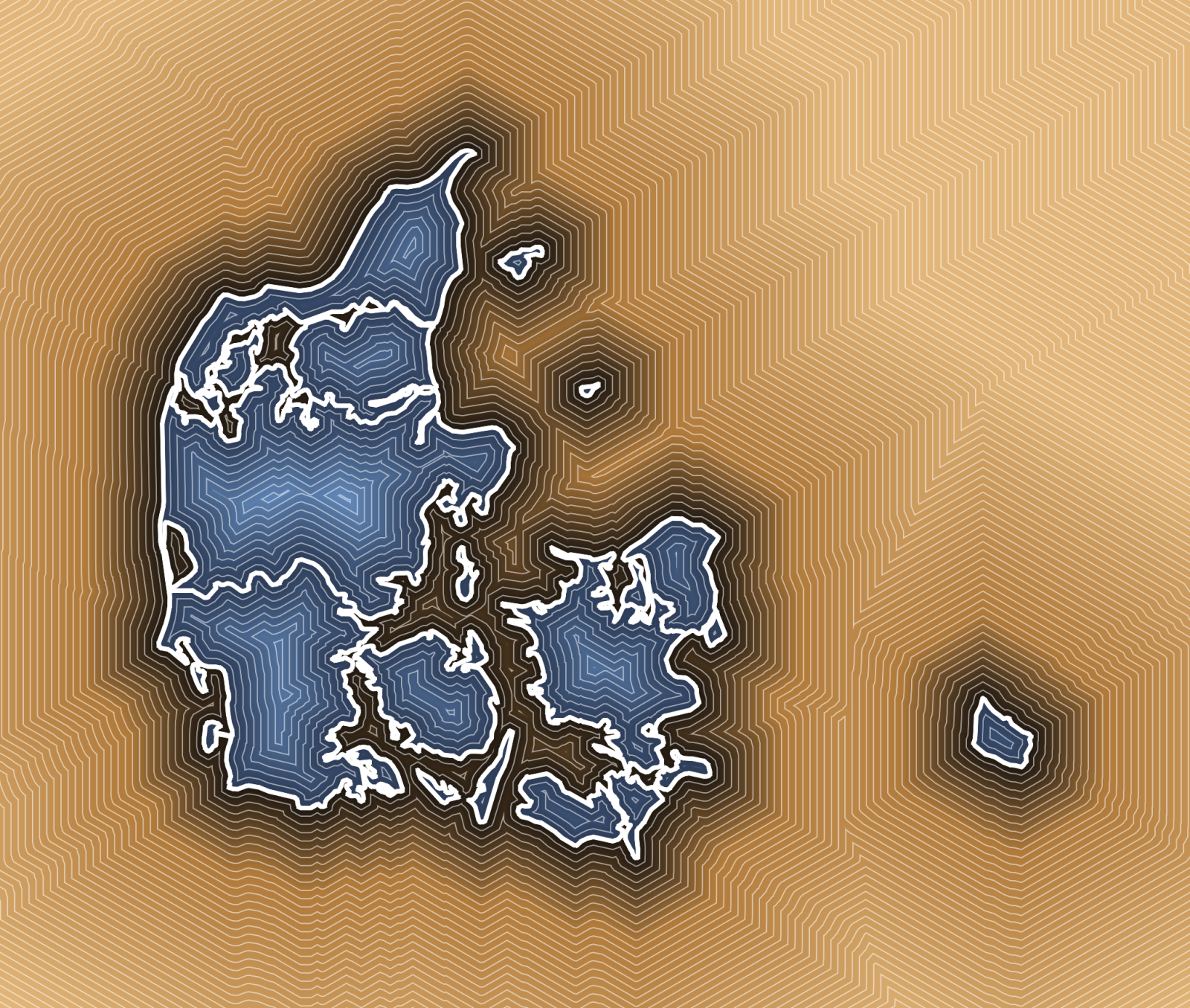
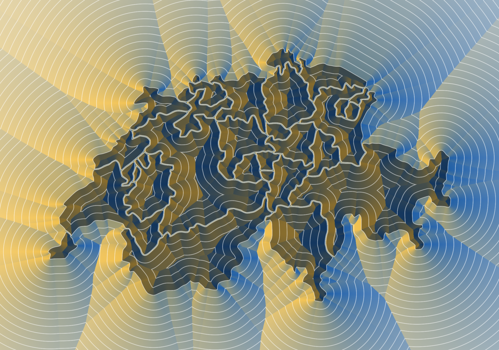
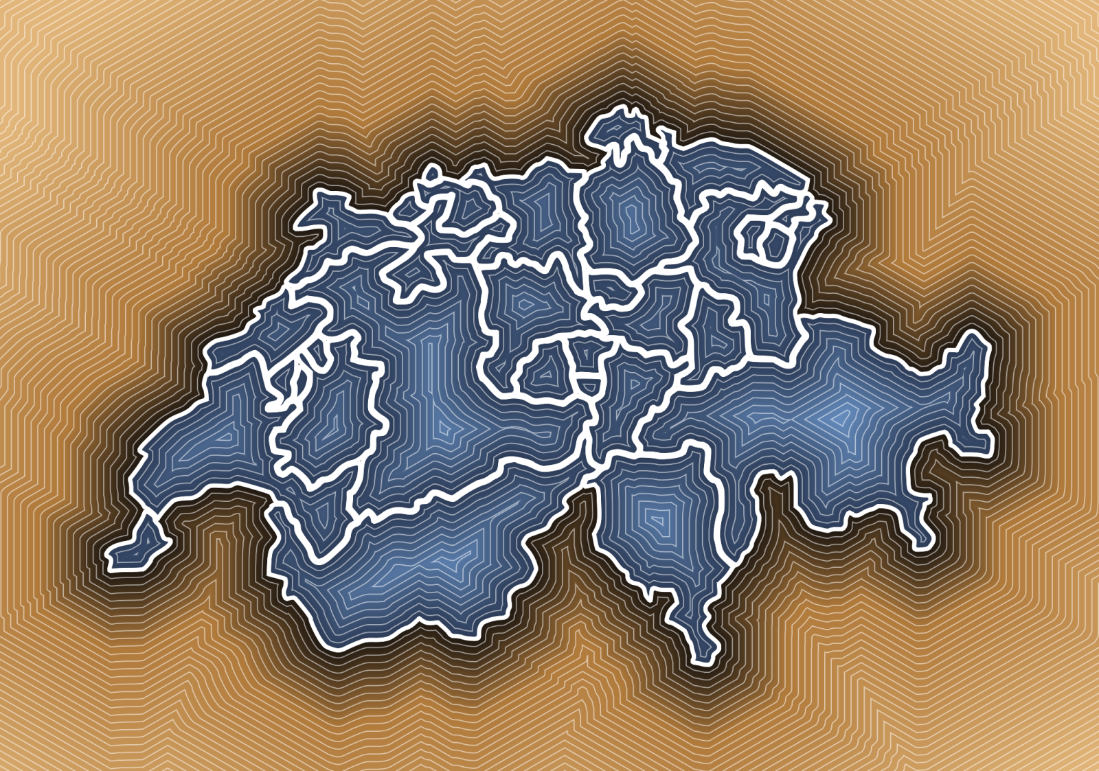
The ramps forget about direction and only color by distance, which gives the more familiar look of a contour map. All nine images are the very same buffer of the north of Jutland, only the reading changes - which is pretty much the point of keeping the computation and the coloring apart.
Compute
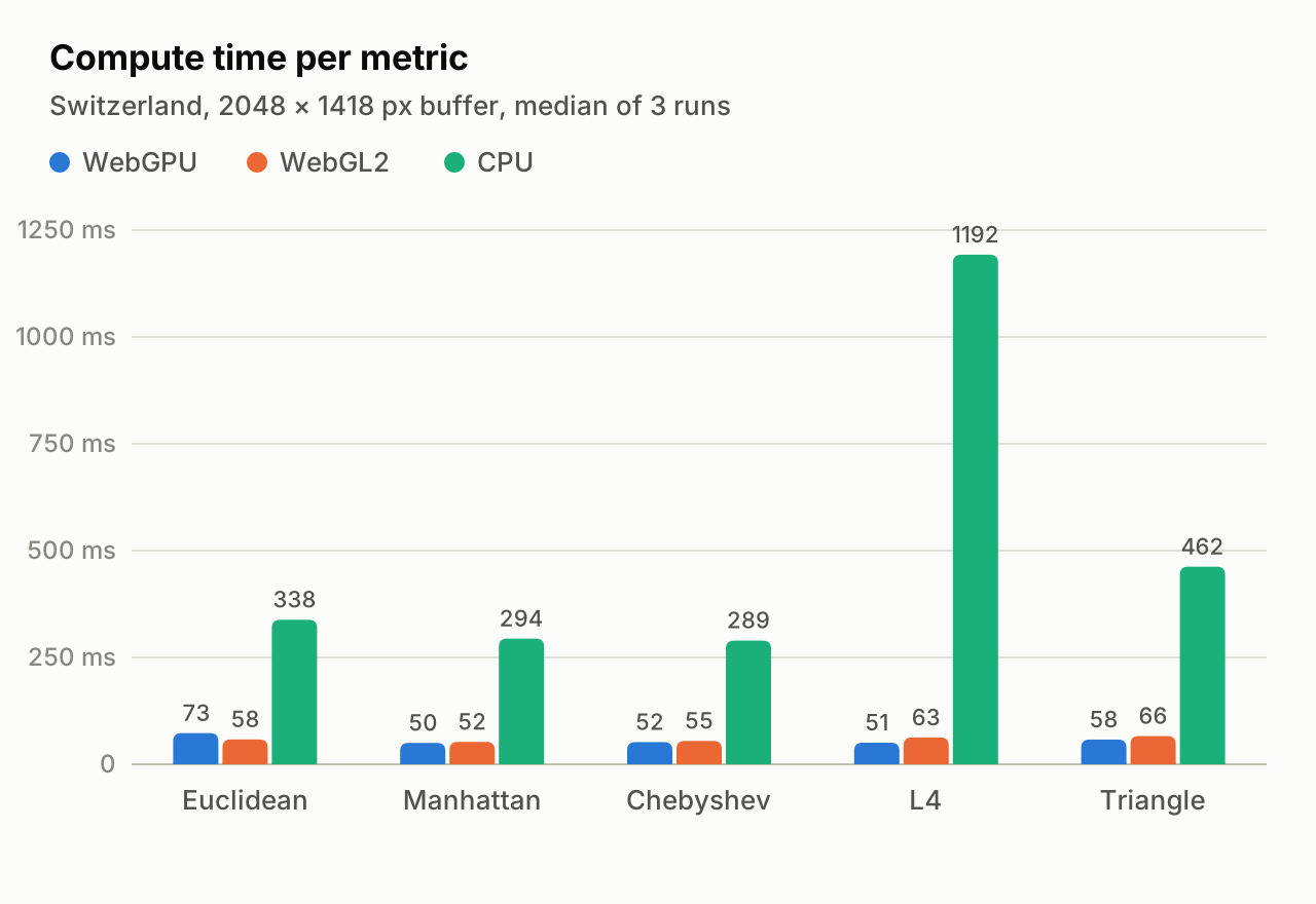
Changing the coloring is instant, changing the metric or the resolution means computing the buffer again. That search runs on WebGPU as a compute shader, on WebGL2 as a fragment shader, or on the CPU with up to 8 web workers. The CPU is the reference, the GPU buffers match it to within about 1e-4 of a pixel.
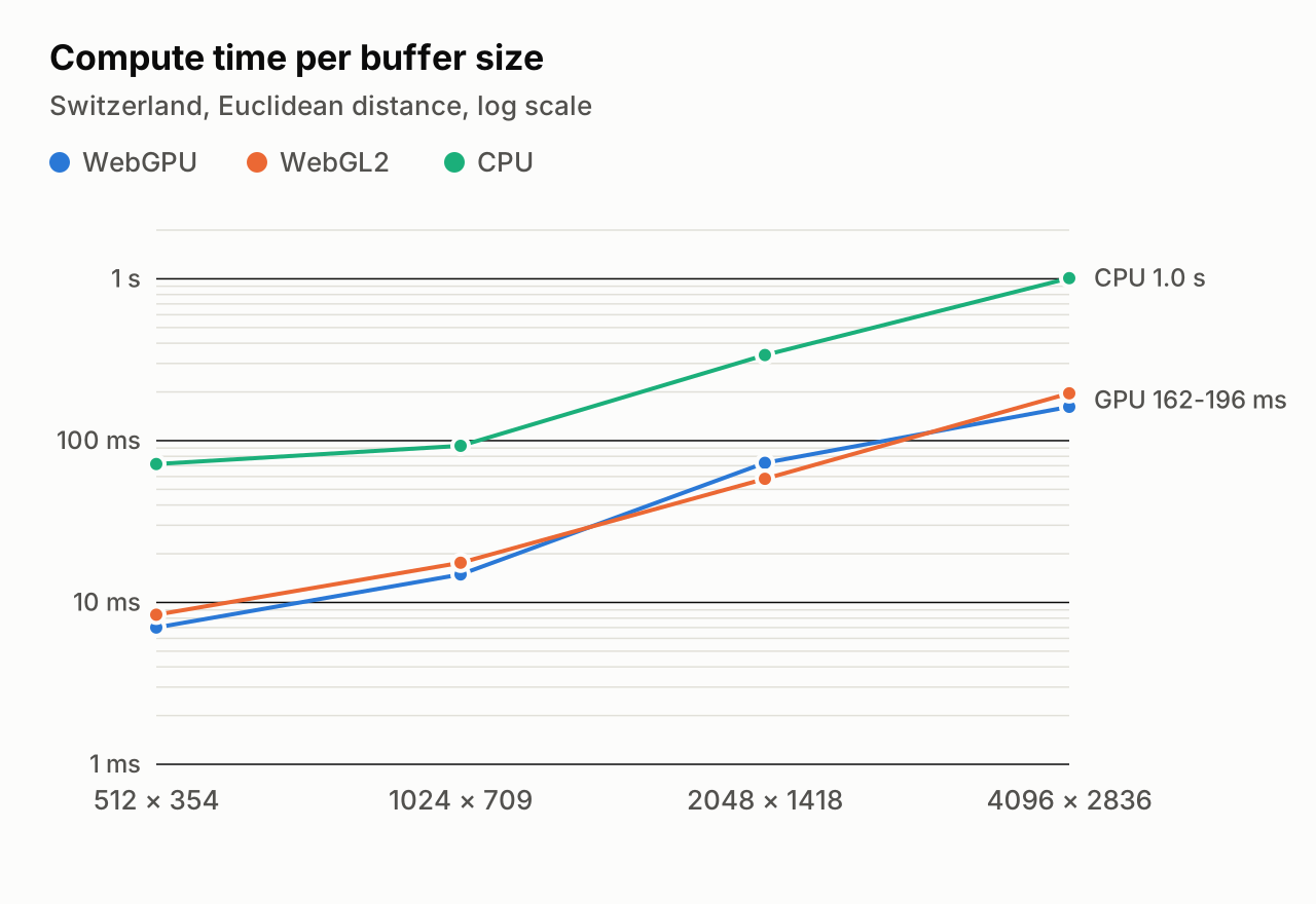
On a MacBook Air with an M4, in Chrome and with the Swiss outline, both GPU paths need 50 to 73 ms for a 2048 px buffer, the CPU workers between 289 ms and 1.2 s. That is the difference between trying out a metric and waiting for one. WebGPU and WebGL2 end up pretty much equally fast. Also precision needed some care: map coordinates are large numbers and float32 does not like large numbers, so the geometry is first moved around the centre of the buffer.
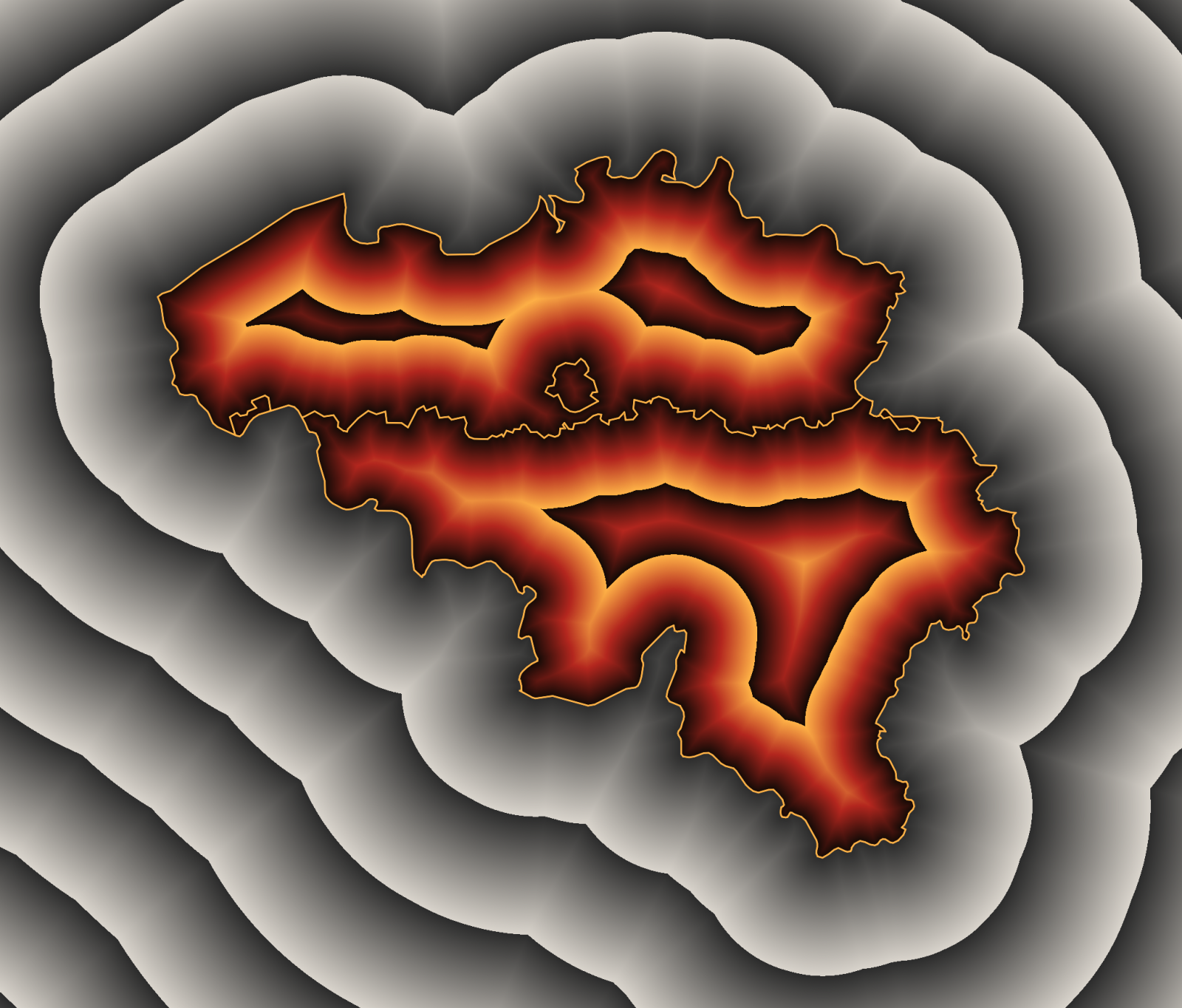
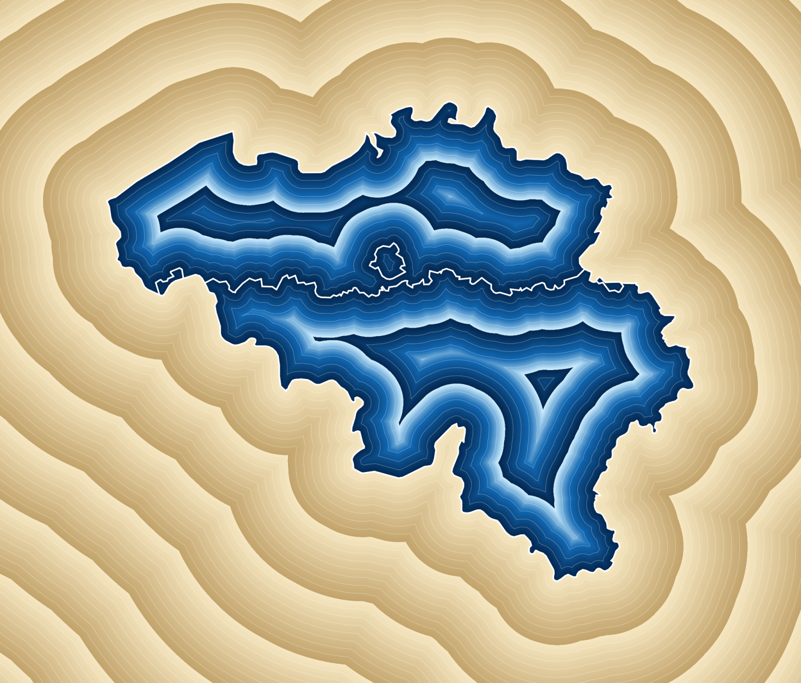
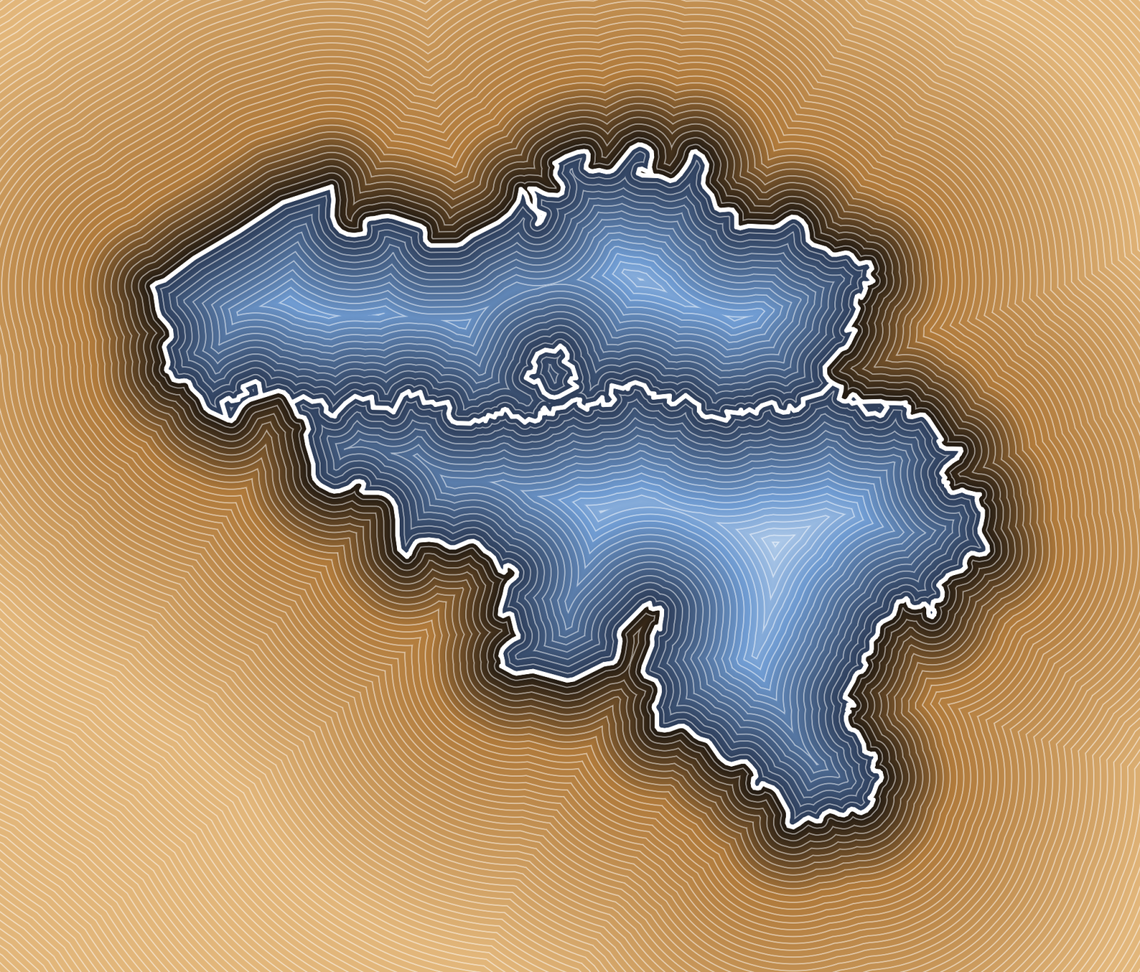
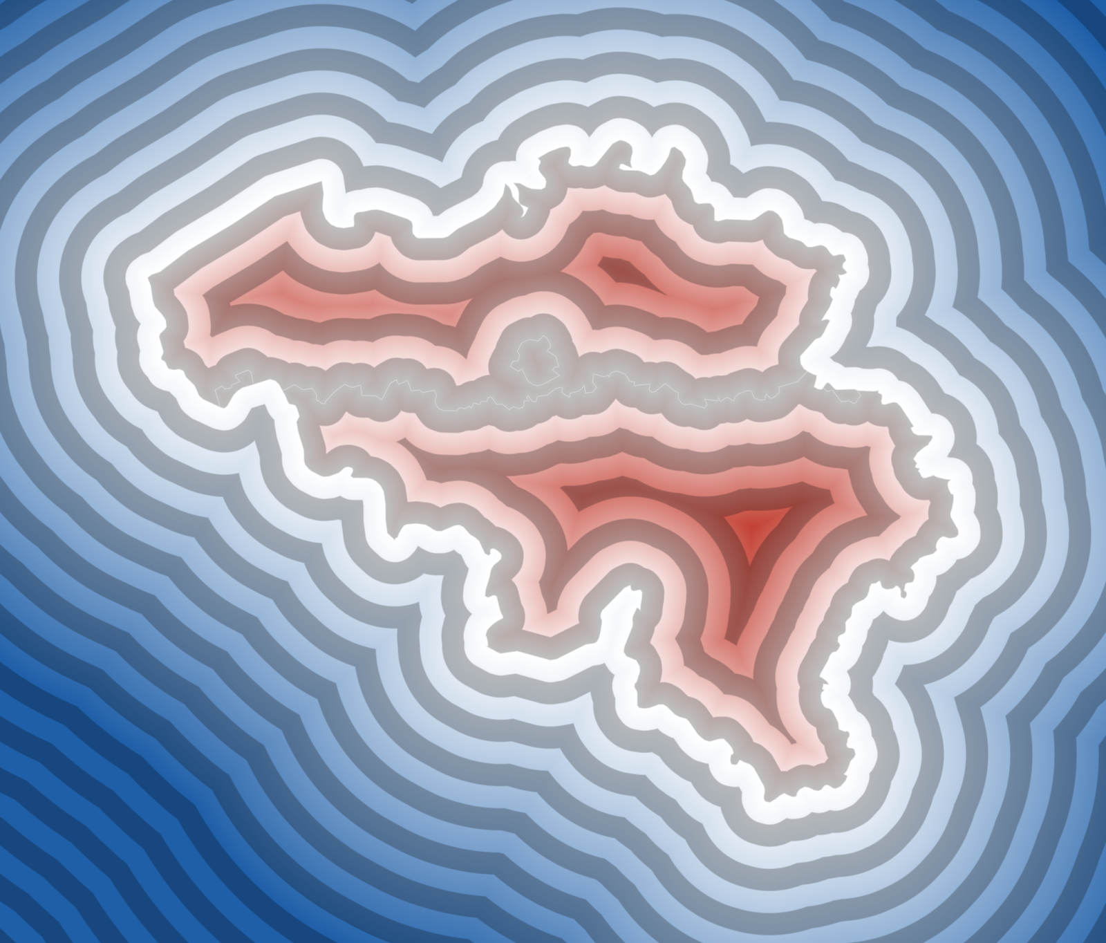
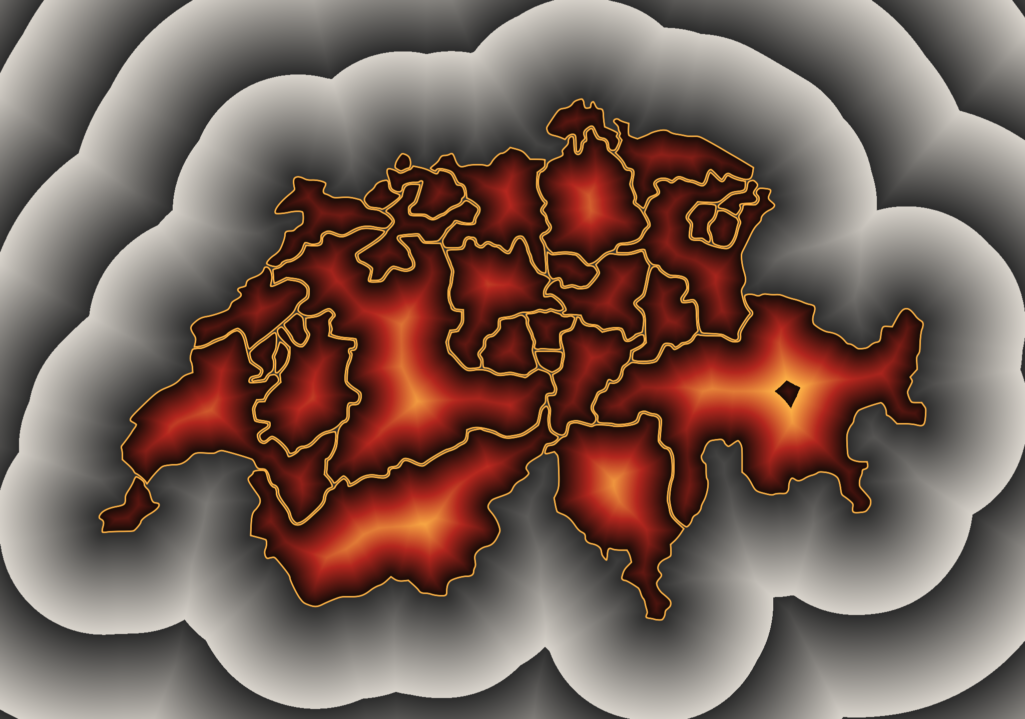
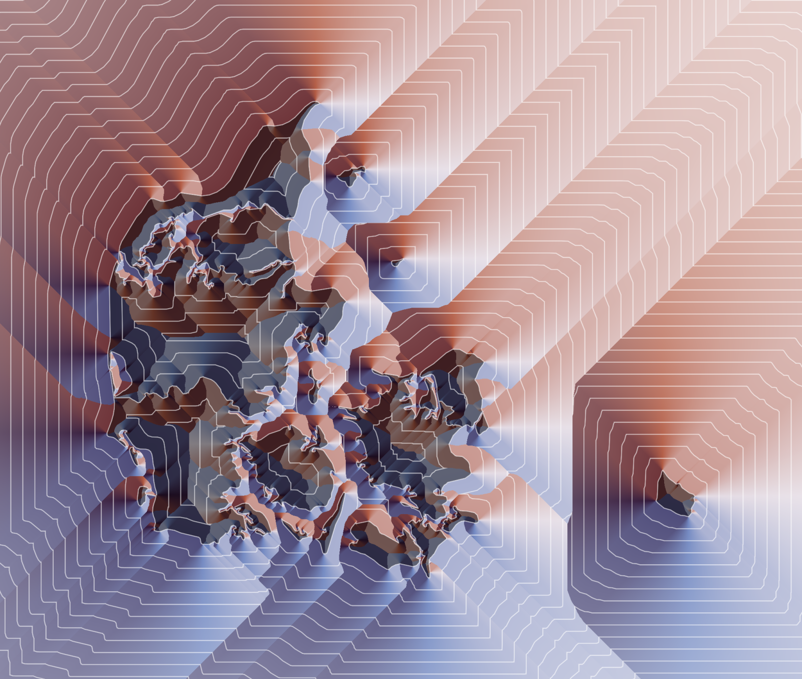
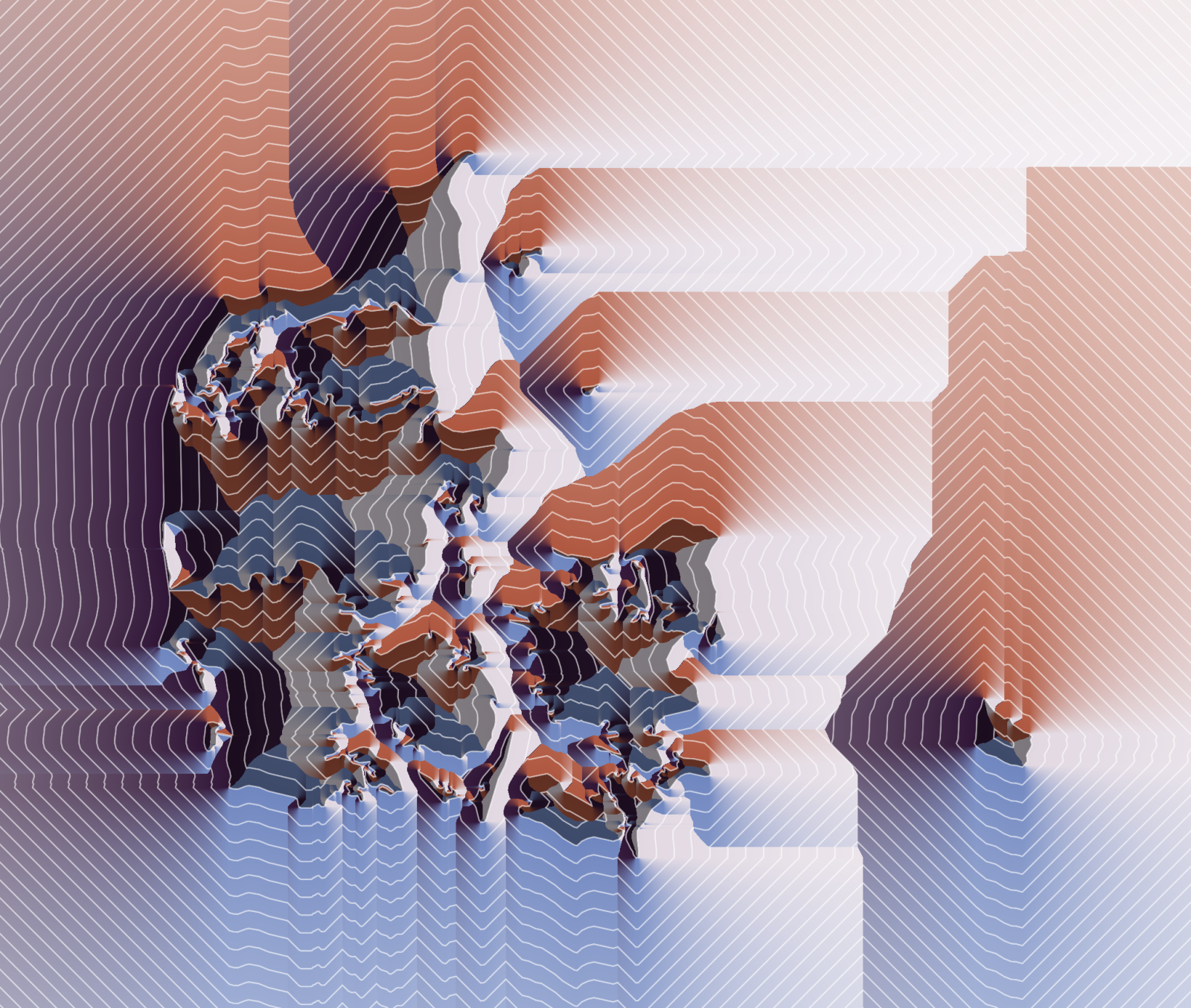
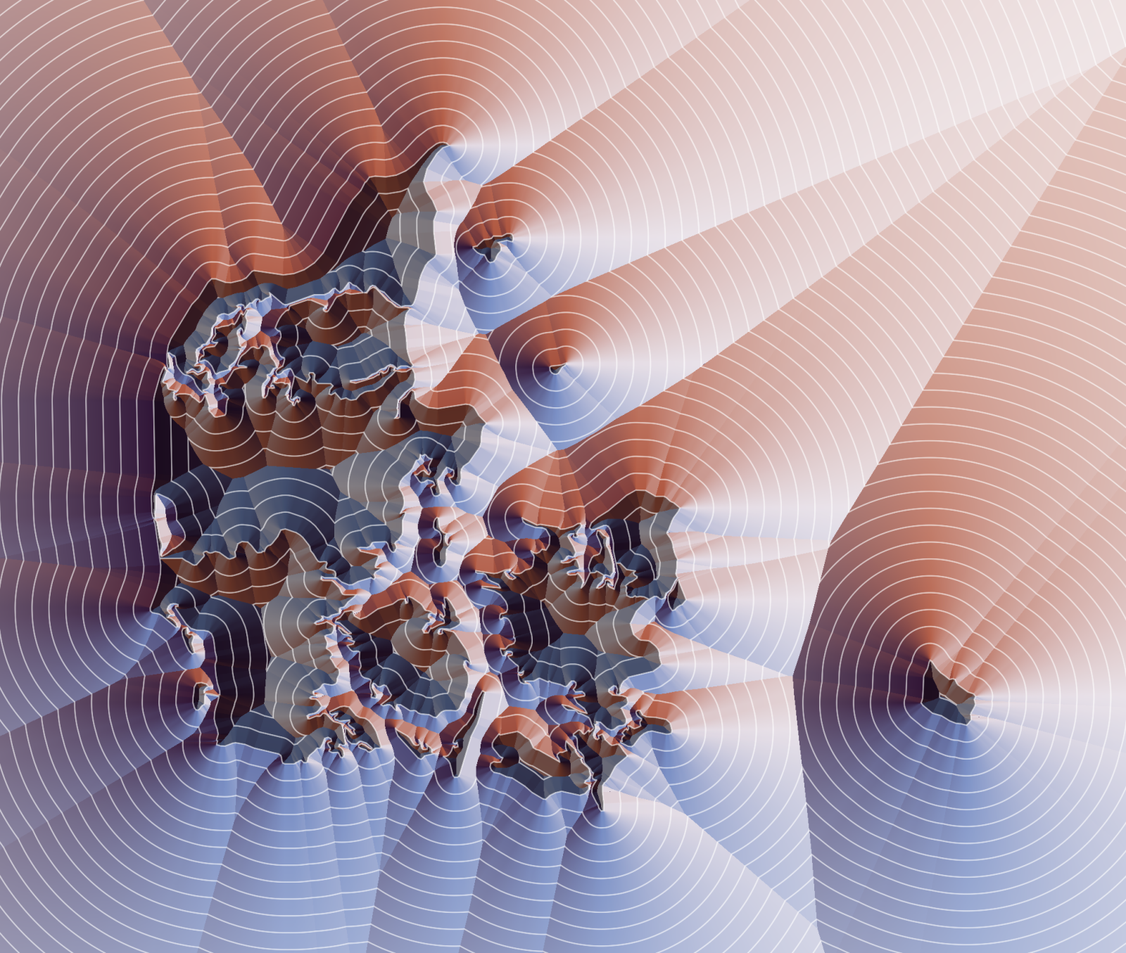
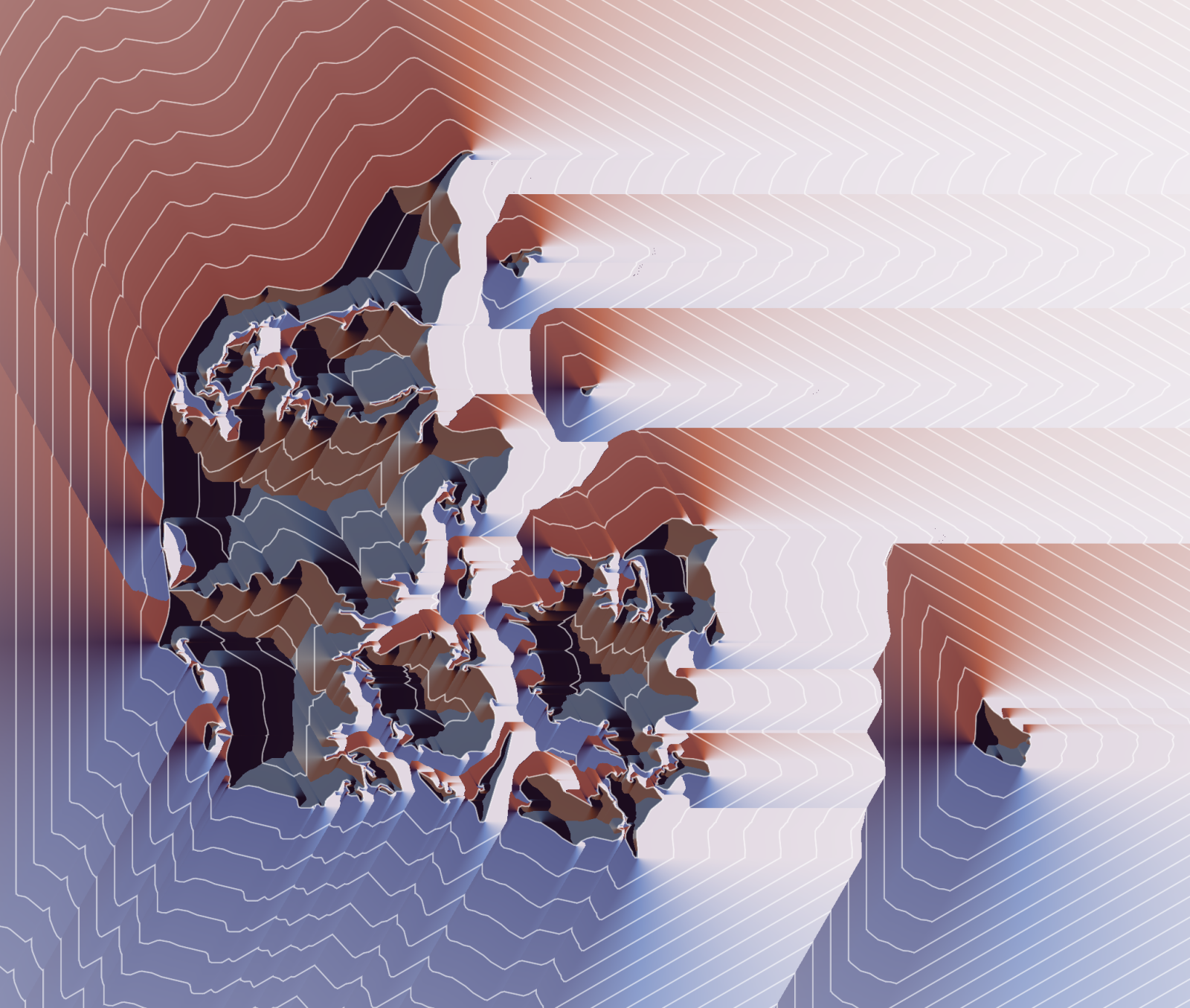
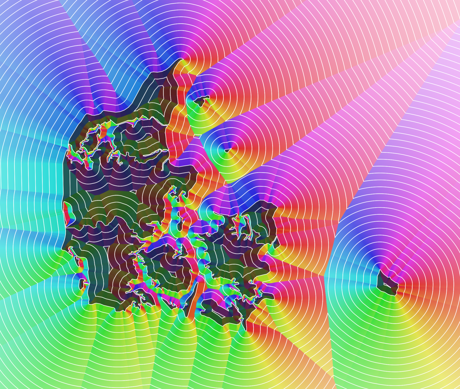
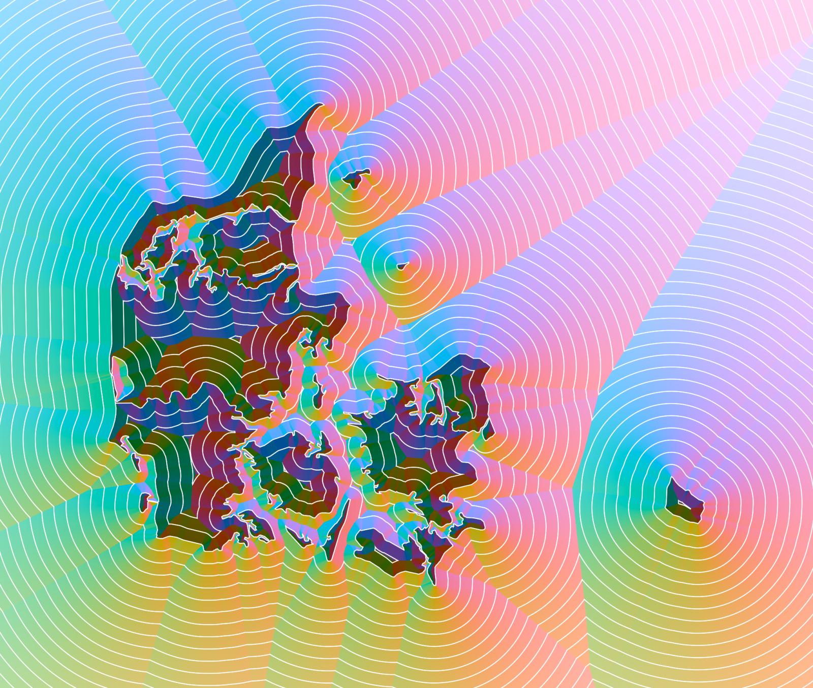
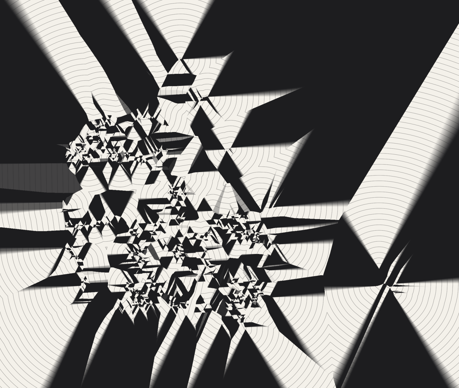
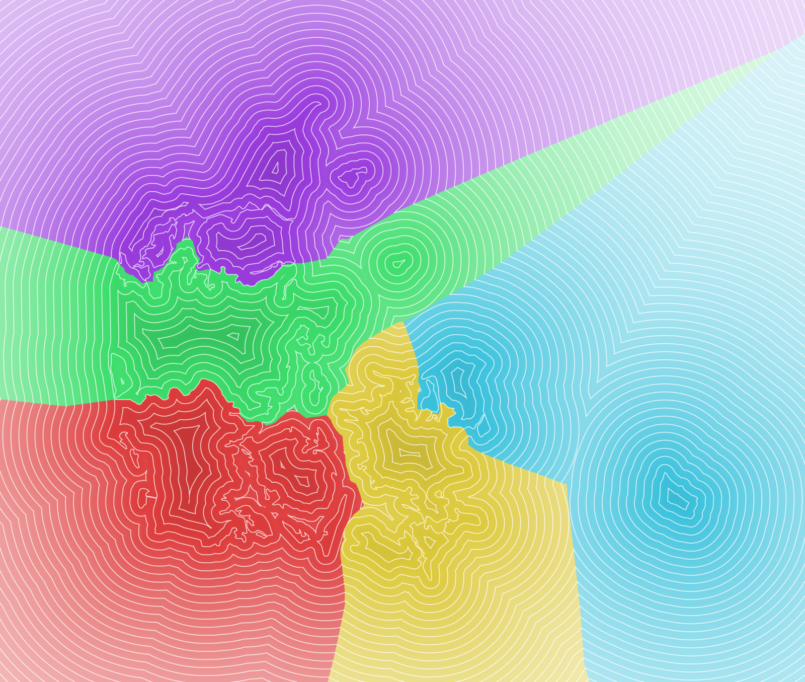
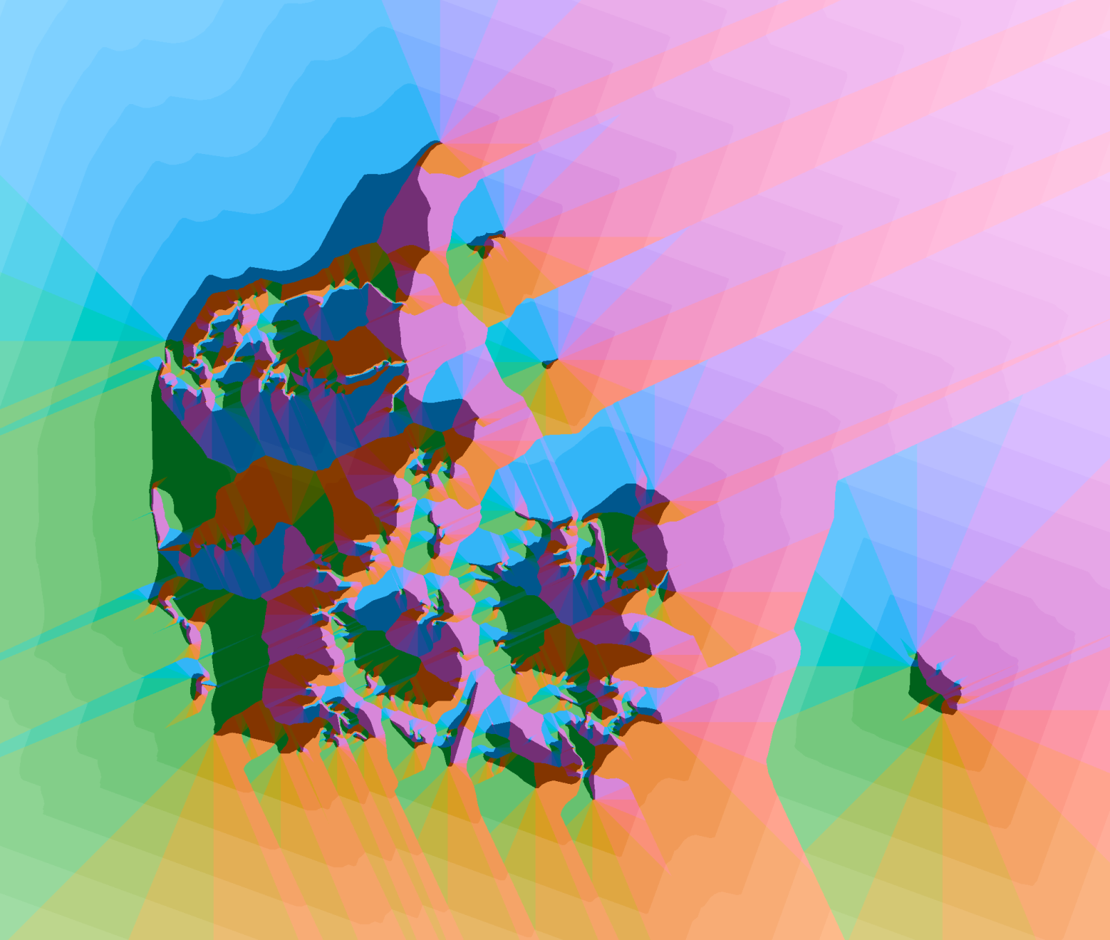
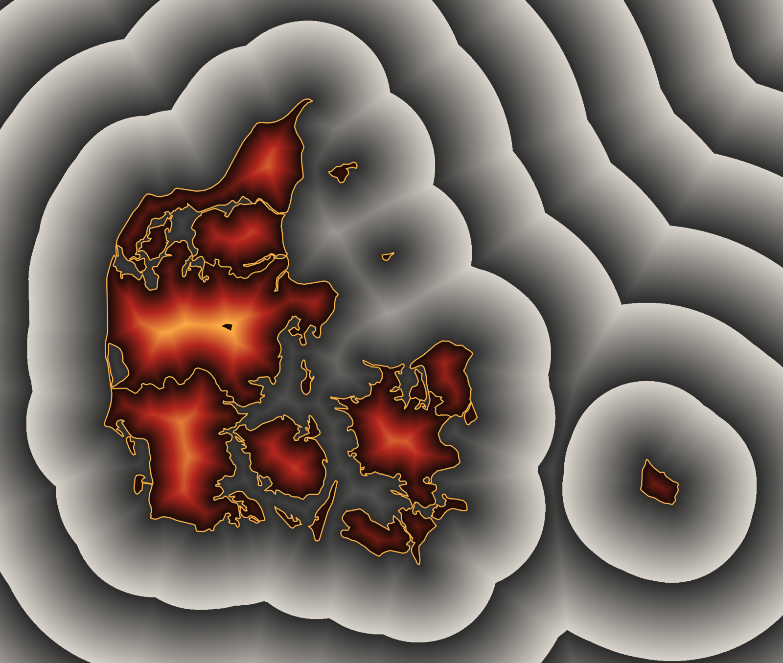
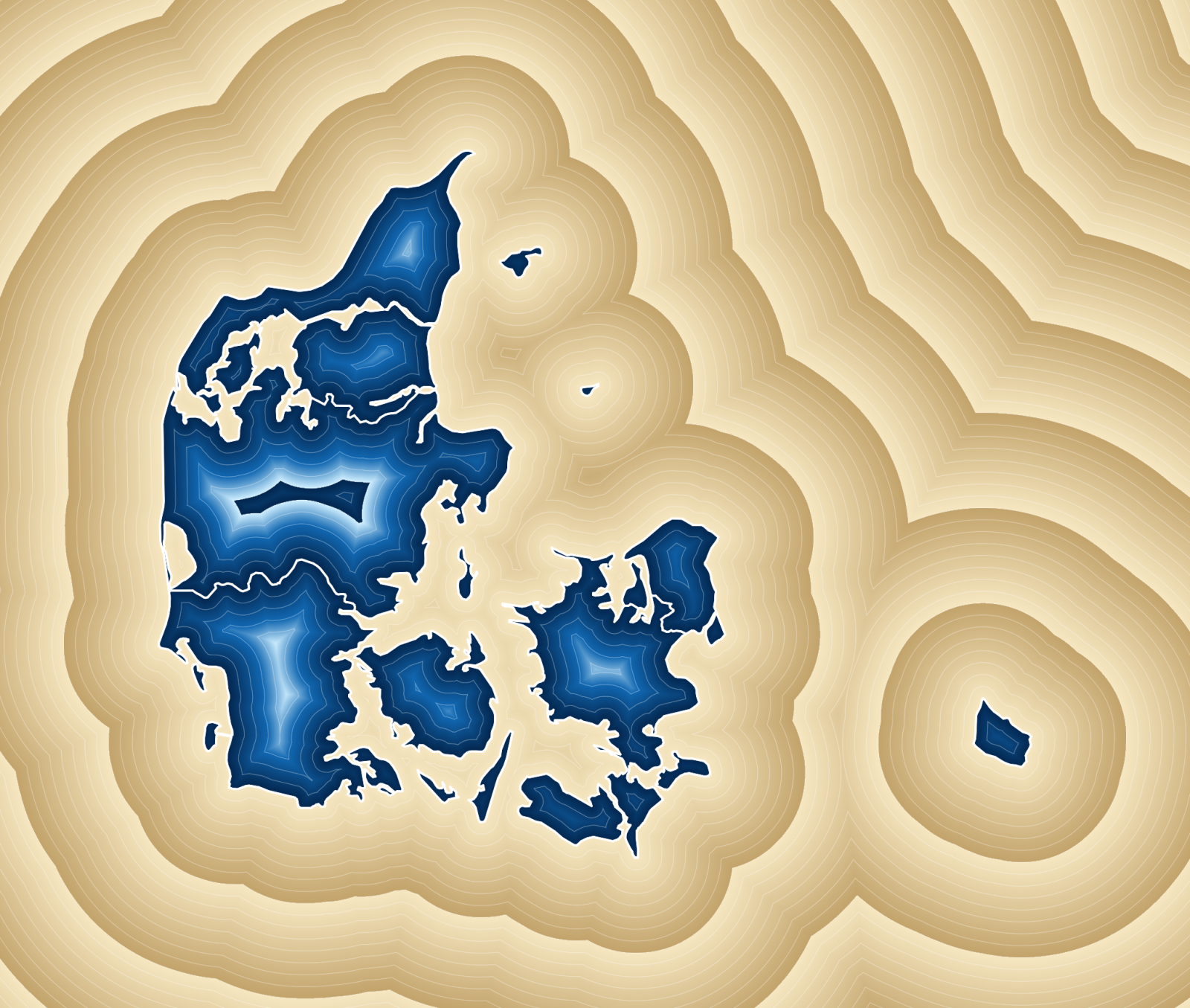
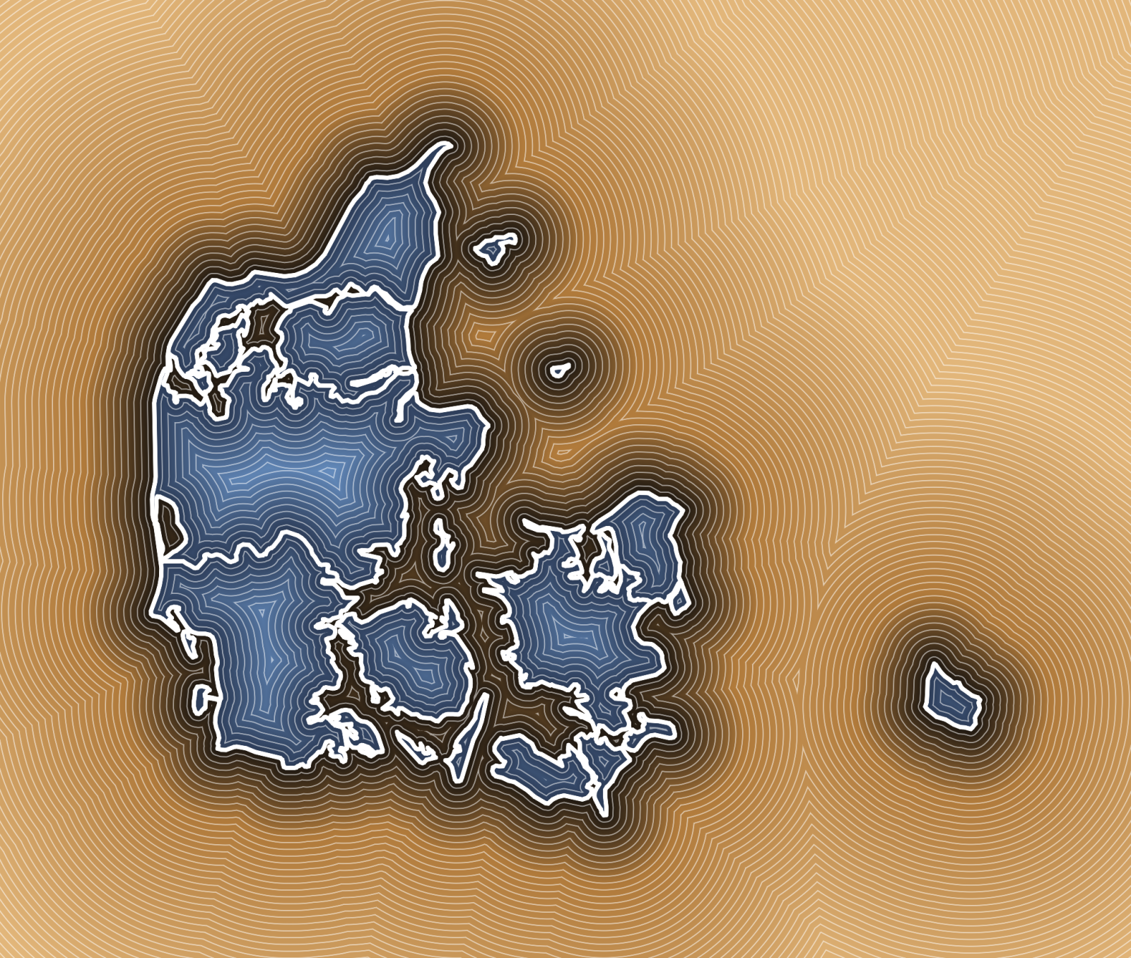
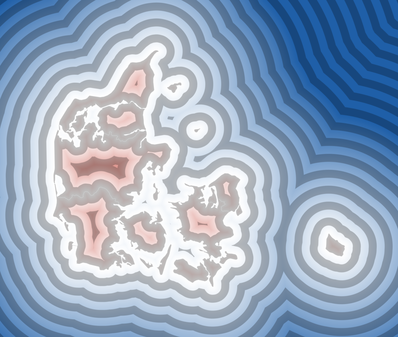
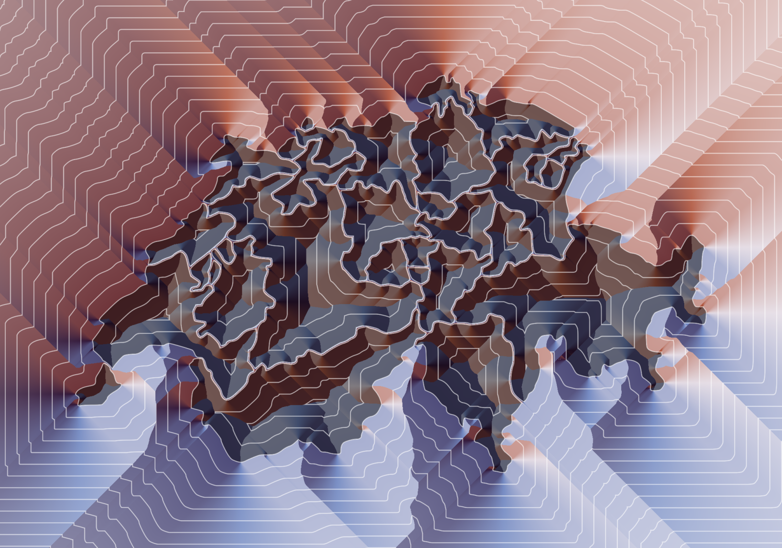
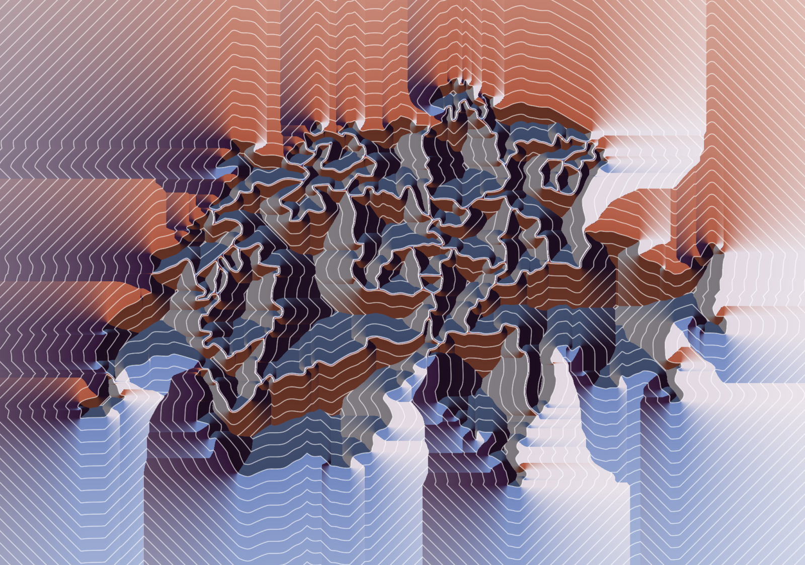
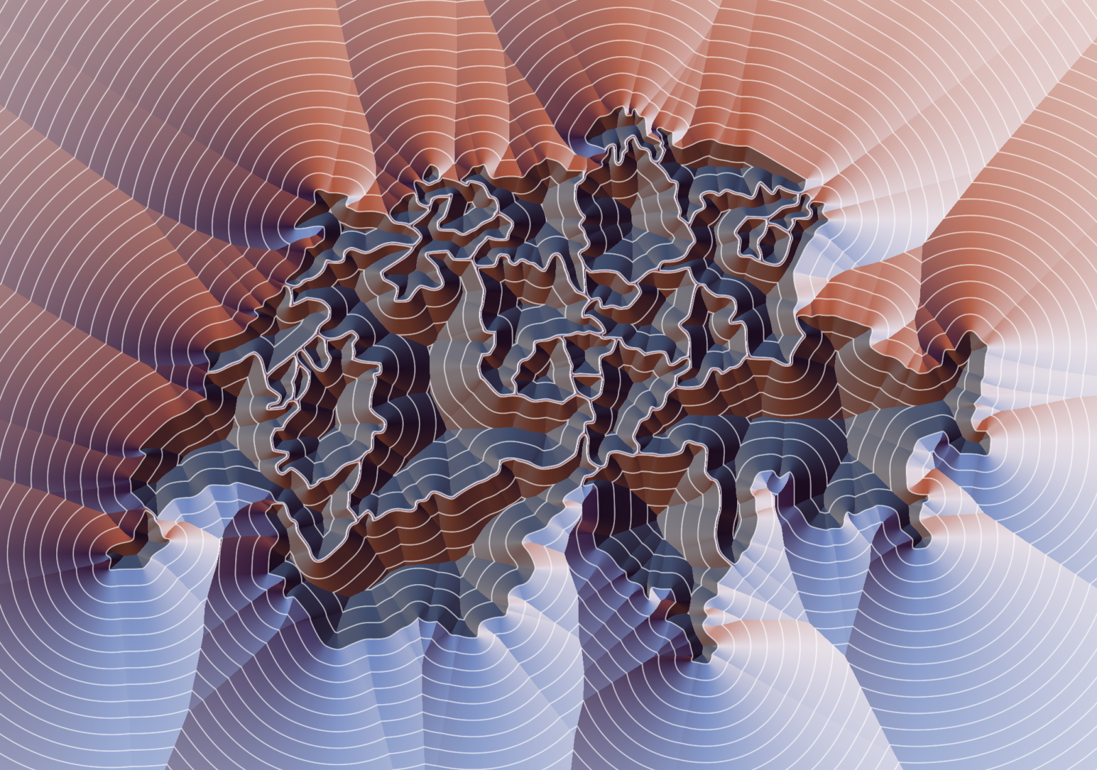
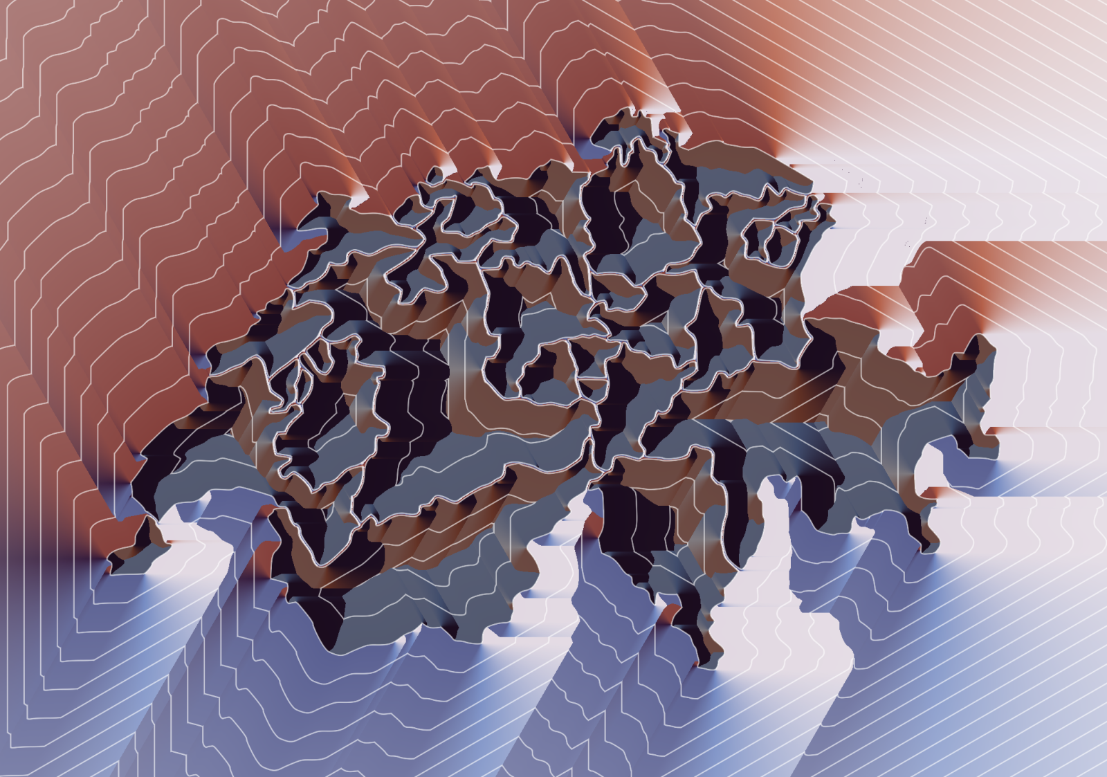
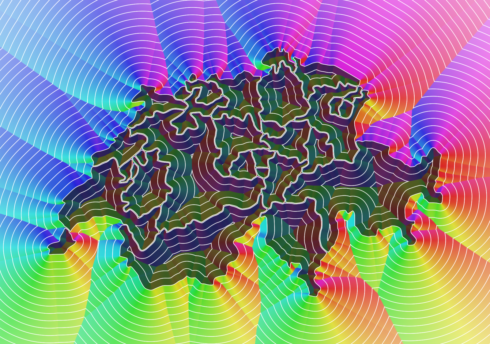
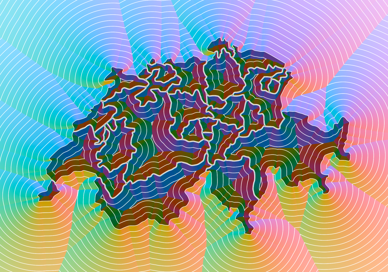
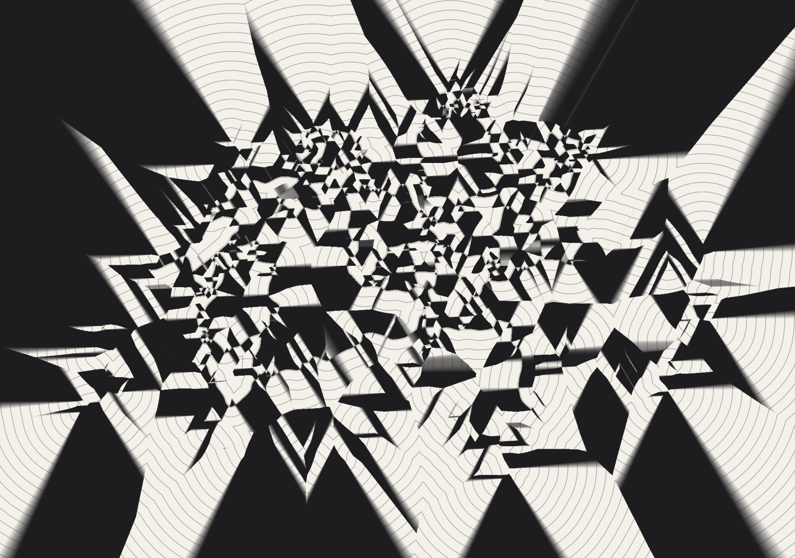
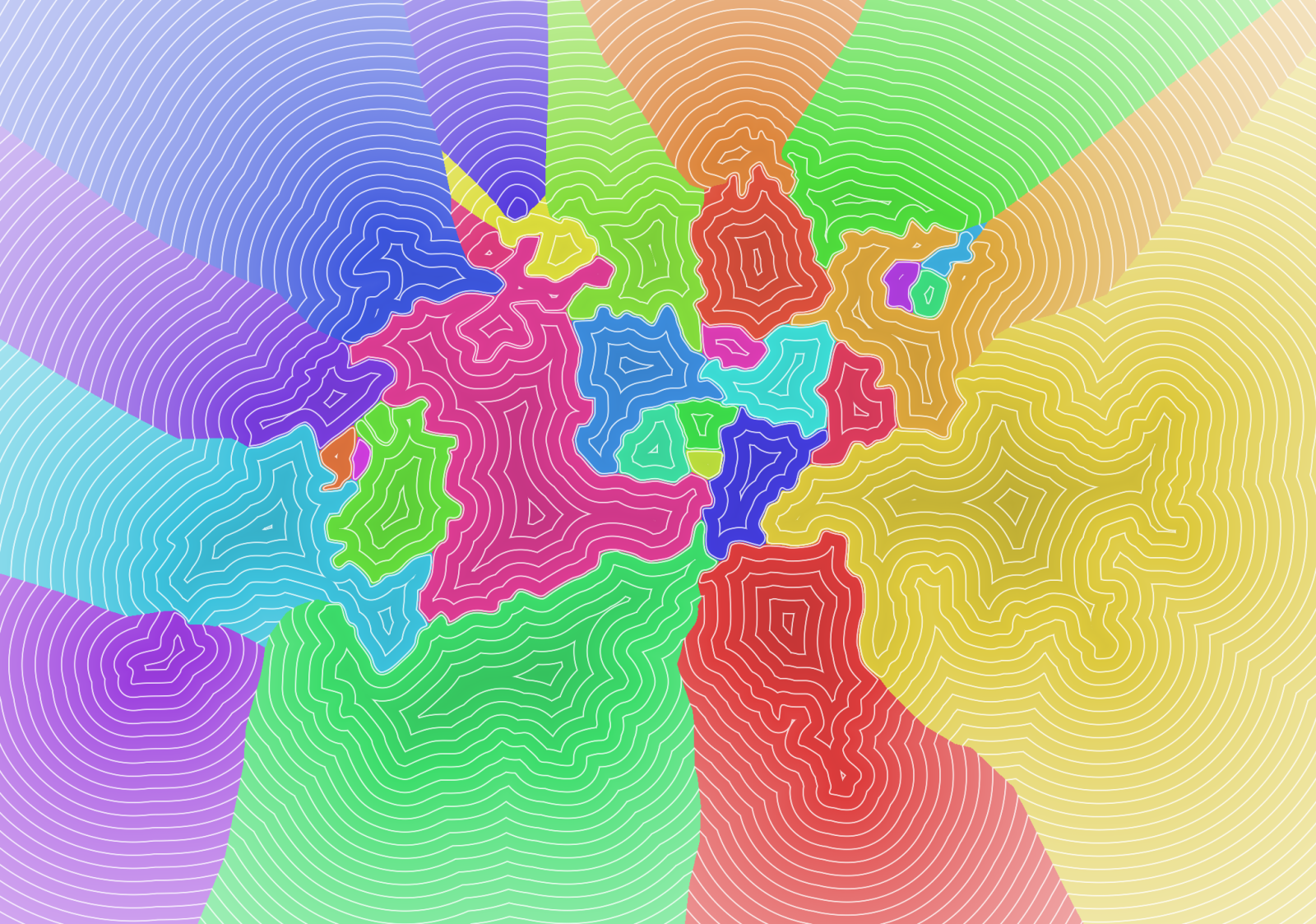
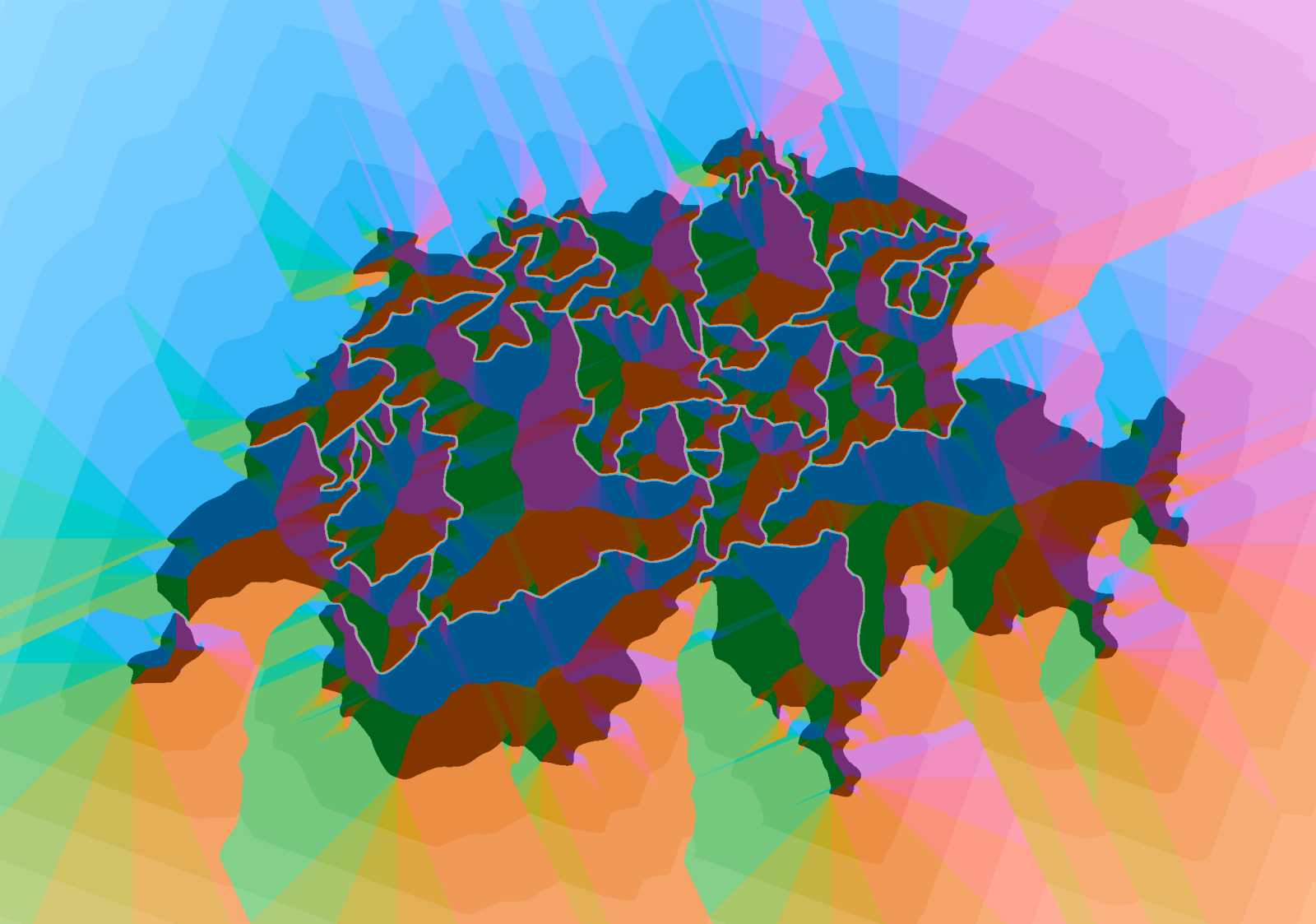
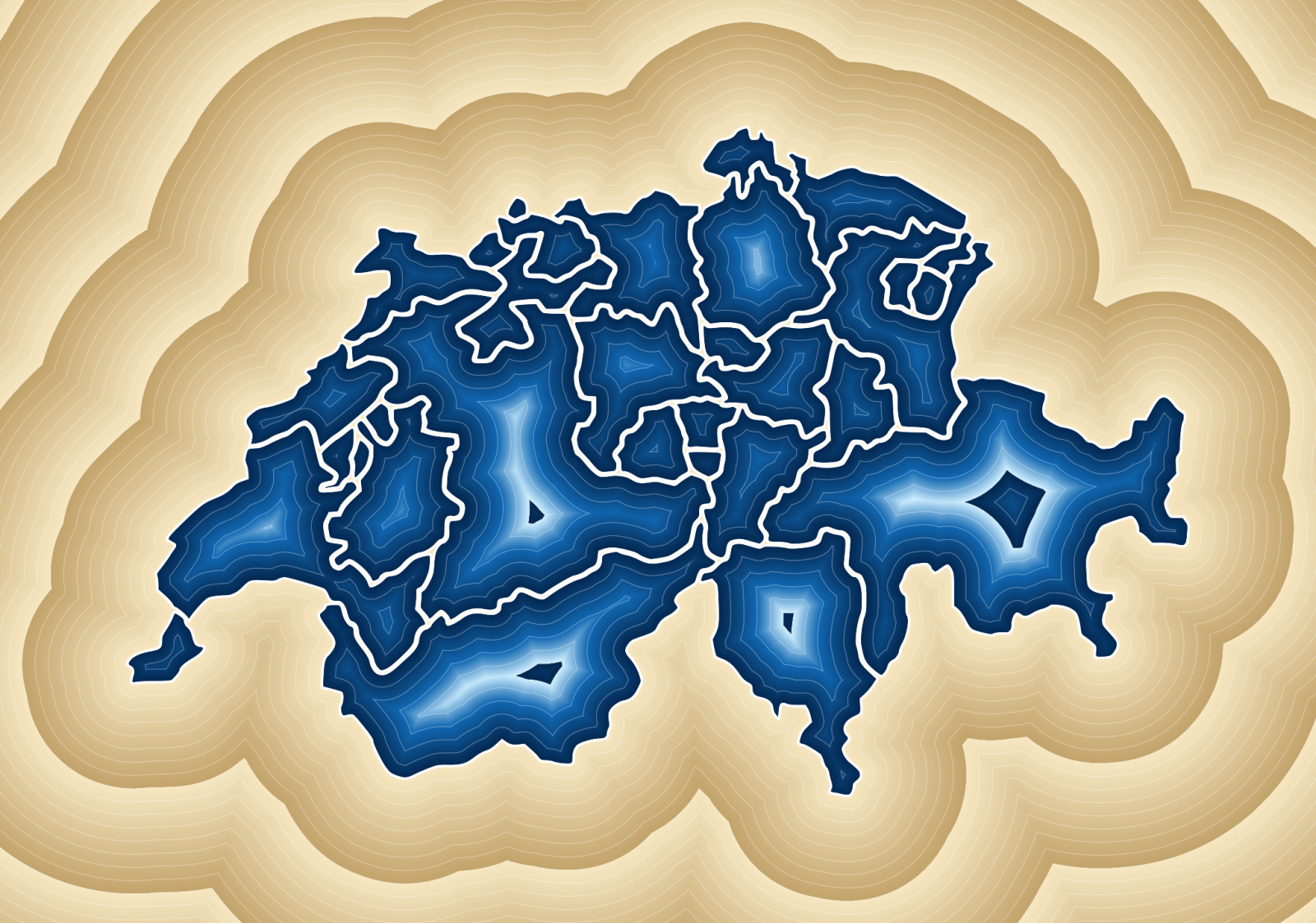
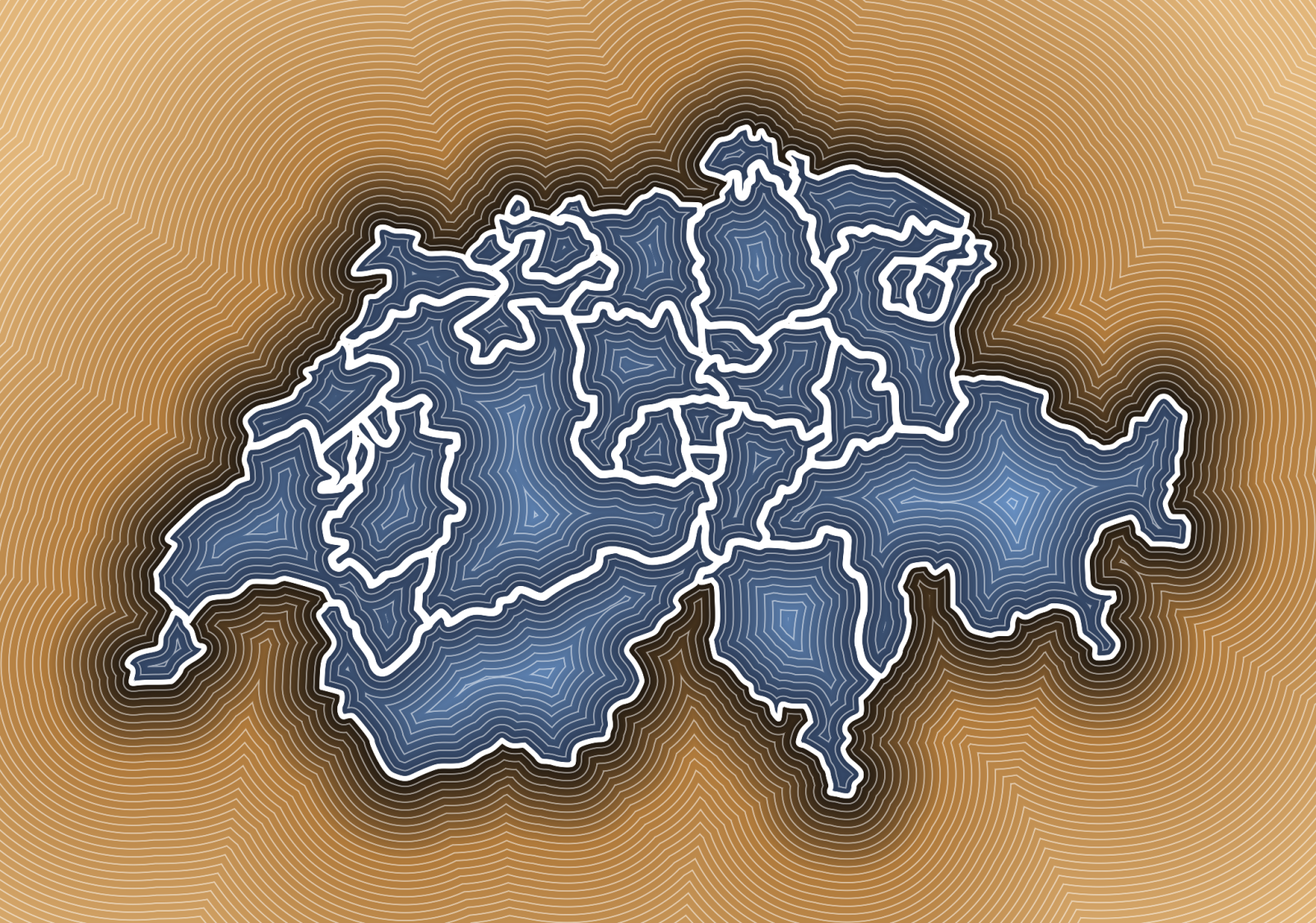
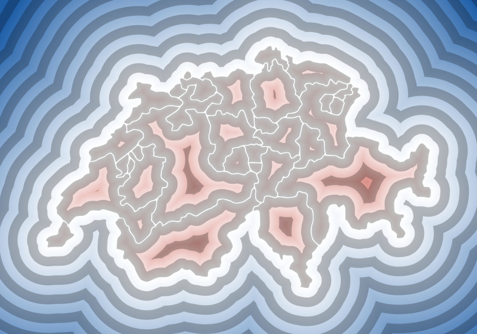
Denmark, Switzerland and Belgium, each with the same sixteen colorings and metrics. Borders make for rather good drawings to start from. They are found lines, drawn by history rather than by a designer, full of islands, enclaves and coasts that never run straight. Run through a distance field they turn into landscapes, with the ridges on the lines furthest away from any border.
Denmark
Lots of islands, and every one of them pulls on the field around it, so the sea in between turns into a maze of seams. The outline is from simplemaps.com.
Switzerland
The only one of the three drawn with actual curves, over 1300 cubic Béziers. The cantons are all one single path, so to give each its own color they first had to be split up.
Belgium
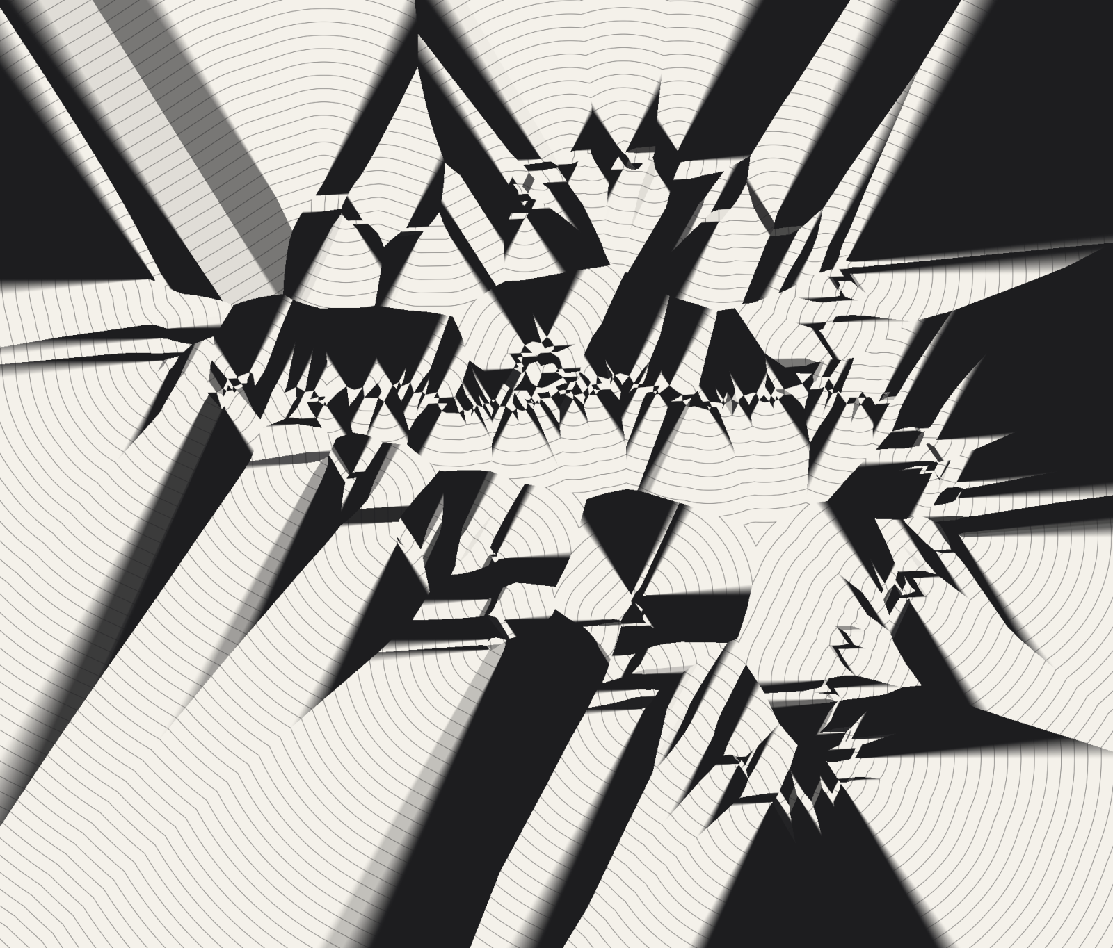
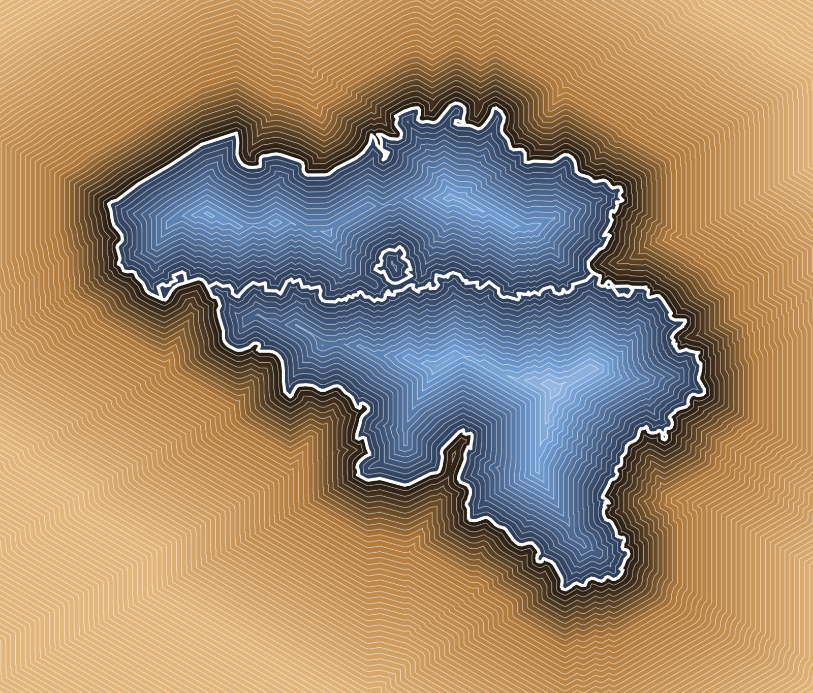
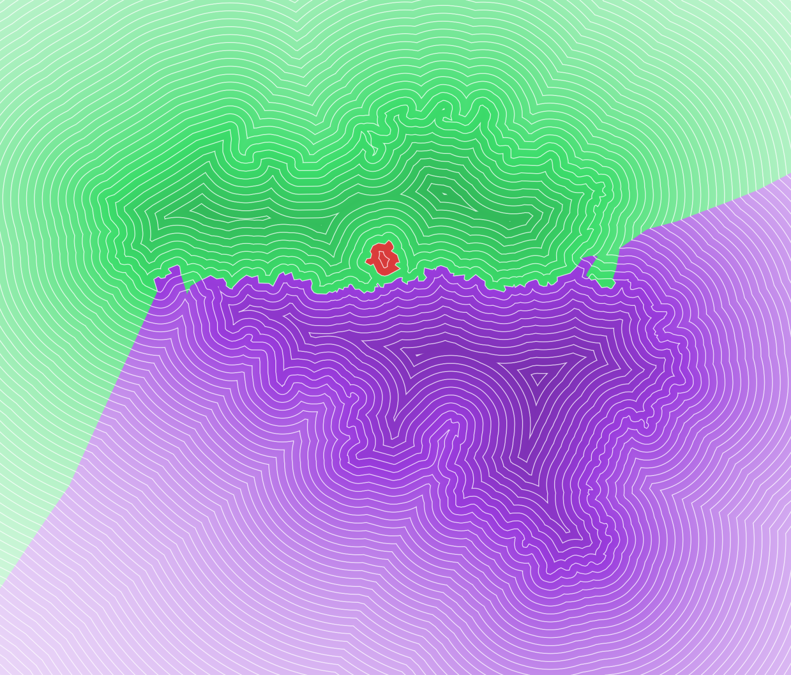
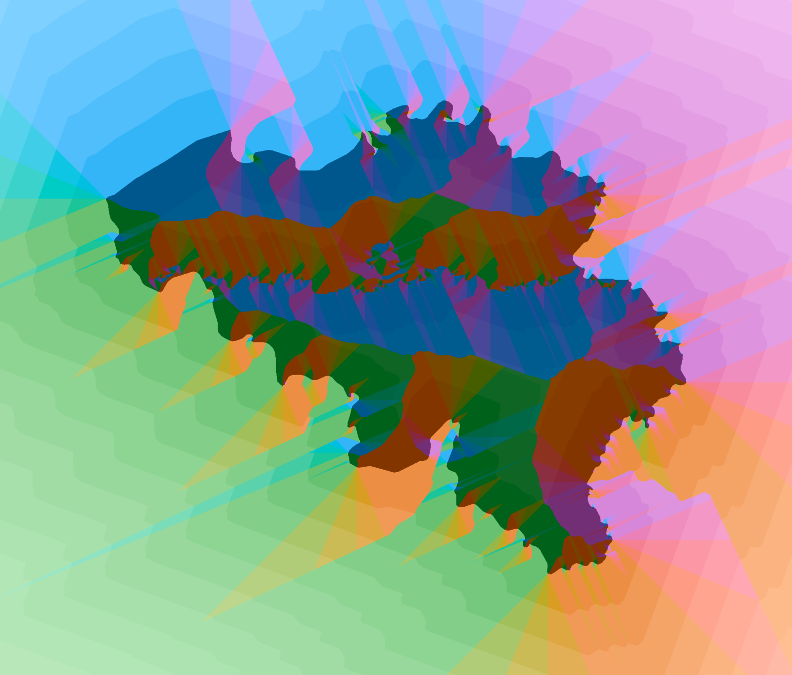
Three regions - Flanders, Wallonia and Brussels - and not a single curve, so every coloring by direction comes out in flat facets. The outline is from simplemaps.com.